
3D Transient Excitations (Sources)
In the 3D transient (time domain), the solver uses the  formulation. The default order of the magnetic scalar potential is 2 and the default order of the electric vector potential is 1. Motion
(translational or cylindrical/non-cylindrical rotation) is allowed, excitations
- currents and/or voltages- can assume arbitrary shapes as functions
of time, nonlinear BH material dependencies are also allowed. The support
of voltage excitations for the windings has as consequence the fact that
the winding currents are unknown and thus the formulation has to be modified
slightly to allow Maxwell to account for source fields due to unknown
currents in voltage - driven solid conductors (where eddy effects are
evaluated) and in voltage-driven stranded conductors -where the eddy
effects (such as skin and proximity effects) are ignored. Also for a
simpler formulation of problems where motion is involved, Maxwell uses
a particular convention and uses the fixed coordinate system for the
Maxwell's equations in the moving and the stationary part of the model.
Thus the motion term is completely eliminated for the translational type
of motion while for the rotational type of motion a simpler formulation
is obtained by using a cylindrical coordinate system with the z axis
aligned with the actual rotation axis.
formulation. The default order of the magnetic scalar potential is 2 and the default order of the electric vector potential is 1. Motion
(translational or cylindrical/non-cylindrical rotation) is allowed, excitations
- currents and/or voltages- can assume arbitrary shapes as functions
of time, nonlinear BH material dependencies are also allowed. The support
of voltage excitations for the windings has as consequence the fact that
the winding currents are unknown and thus the formulation has to be modified
slightly to allow Maxwell to account for source fields due to unknown
currents in voltage - driven solid conductors (where eddy effects are
evaluated) and in voltage-driven stranded conductors -where the eddy
effects (such as skin and proximity effects) are ignored. Also for a
simpler formulation of problems where motion is involved, Maxwell uses
a particular convention and uses the fixed coordinate system for the
Maxwell's equations in the moving and the stationary part of the model.
Thus the motion term is completely eliminated for the translational type
of motion while for the rotational type of motion a simpler formulation
is obtained by using a cylindrical coordinate system with the z axis
aligned with the actual rotation axis.
The formulation used by the Maxwell transient module supports Independent-Dependent boundary conditions and motion induced eddy currents everywhere in the model, in the stationary as well as in the moving parts of the model. Mechanical equations attached to the rigid-body moving parts allows a complex formulation with the electric circuits being strongly coupled with the finite element part and also coupled with the mechanical elements whenever transient mechanical effects are included by users in the solution. In this case the electromagnetic force / torque is calculated using the virtual work approach. For problems involving rotational type of motion a "sliding band" type of approach is followed and thus no re-meshing is done during the simulation. For translational type of motion the mesh in the band object (surrounding the part in motion) needs to be re-created at each timestep with a degree of refinement which is dependent upon the mesh size in the moving object. In this later case the mesh in both stationary and moving objects remains unchanged as initially created by the user. For transient type of electromagnetic field analysis (with or without motion) the user is responsible for creating the mesh that is capable to "catch" the respective physics such as skin and proximity effects -if any- are to be present in the resulting fields.
The following three Maxwell's equations are relevant for transient (low frequency) applications:


The following two equations directly result from the above equations:


The final result is a formulation where vector fields are represented by first order edge elements and scalar fields are represented by second order nodal unknowns.
Field equations are coupled with circuit equations for both solid and stranded conductors because, in the case of applied voltage supplies, the currents are unknown. For the case of voltage driven solid conductors, the following equation is used to account for the ohmic drop across the i-th conductor loop:
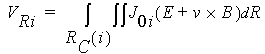
where J0i represents the current density.
The current density J0i corresponds to 1A of net current in loop i and vanishes outside loop i.
The induced voltage can be derived from the following equation:
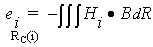
where the integration is performed over the whole conductor region.
Stranded conductors are considered to be without induced eddy currents and, thus, are placed in the non-conducting region. This means that, for the purpose of calculating the ohmic voltage drop, the procedure for solid conductors cannot be used. Instead, a lumped parameter is used to represent the DC resistance of the winding. The induced voltage due to the total flux linkage is obtained in a similar way as for solid conductors. In both cases, it is also possible to add an external inductance and capacitance.
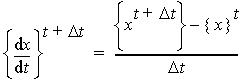
For the time discretization, a backward time-stepping scheme is used:
For the nonlinearities allowed in 3D transient applications, the classical Newton-Raphson algorithm is used.
The transient solver in Maxwell supports the coil terminals and winding definitions. Thus it is possible to specify the number of turns of coils in models which is necessary for the calculation of global quantities with high engineering value such as flux linkage and back emf of coils. Thus for the 3D transient solver a number of quantities are automatically calculated and displayed as 2D plots (functions of time): voltage (current), flux linkage, back emf. Other global quantities can be also calculated by the 3D transient solver and displayed as 2D plots such as power loss, core loss, stranded loss, electromechanical quantities such as force/torque, speed and displacement.
A few types of sources can be used in 3D transient applications. The Coil Terminal type is discussed here.