
IC Packages - Extract Delphi Network
Extract Delphi Network creates, trains, and exports a Delphi-like Surrogate Thermal Model (STM) that is Boundary Condition Independent (BCI) and can be used to emulate the thermal behavior of the IC package.
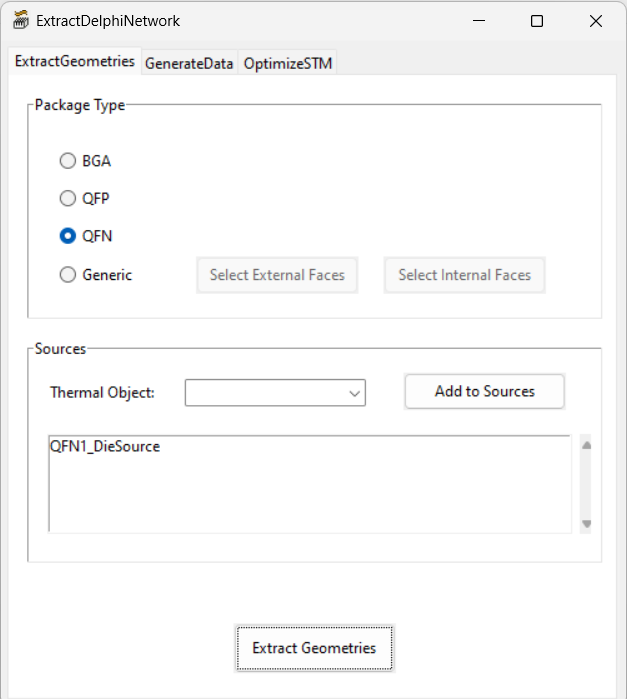
Extract Geometries Tab
The Extract Geometries tab controls the process of selecting specific geometric features from the Detailed Thermal Model (DTM). These features include external faces, internal faces, and heat sources, and they have two primary purposes: to inform the DTM simulations for data production and to fully define the STM’s internal and external geometry.
|
Package Type |
||
|---|---|---|
|
Package Type |
Under Package Type, select the package type for the delphi network extraction. Select Generic for packages that are not BGA, QFP, or QFN created using an Icepak > Toolkits > Geometry toolkit. For generic packages, click Select External Faces to export groups of external faces manually or automatically and Select Internal Faces to manually export groups of internal faces. See External Faces Editor and External Faces Editorfor more information. |
|
|
Sources |
||
|
Thermal Object Add to Sources |
Sources are displayed in the list. If needed, select a thermal object and click Add to Sources to include additional active sources to the resulting network.
|
|
|
|
||
|
Extract Geometries |
Click Extract Geometries to finalize the collection of external faces, internal faces, heat sources, and their related properties. When the process is complete, the Extract Geometries button appears green. |
|
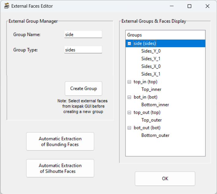
External Faces Editor
In the External Faces Editor, use the External Group Manager to manually create groups of external faces based on geometry selected from the 3D Modeler window or the History tree. Alternatively, you can click Automatic Extraction of Bounding Faces to automatically identify the external faces touching the package's bounding box and categorize them in groups or Automatic Extraction of Silhouette Faces to automatically identify the faces that compose the DTM's silhouette.
| External Group Manager | ||
|---|---|---|
| Group Name |
Enter a Group Name for the group of external face geometry. |
|
|
Group Type |
Enter a Group Type for the group of external face geometry. |
|
|
Create Group |
Click Create Group to save the group name and/or type changes. The Create Group button appears when a group is selected in the Groups tree. |
|
| External Groups & Faces Display | ||
| Group Tree | The External Groups & Faces Display tree lists the groups and associated faces you've created. If needed, select a group and modify its name or type. From a group's right-click menu, you can unite all the faces into one piece of geometry, delete the group, or delete all groups. From an external face's right-click menu, you can split the face, remove it, or move it to a different group. With multiple faces selected, you can split the faces, unite them, remove them, or move them to a different group. | |
|
Automatic Extraction of Bounding Faces |
Click Automatic Extraction of Bounding Faces to automatically identify the external faces touching the package's bounding box and categorize them in groups. After confirming the bounding box selection, the Get Boundaries dialog box appears. Choose whether to create single sheet geometry for each of the six bounding surfaces or to split the sheets into more than one based on the intersecting geometry. Splitting the geometry will require more time to generate all of the geometry. |
|
|
Automatic Extraction of Silhouette Faces |
Click Automatic Extraction of Silhouette Faces to automatically identify the faces that compose the DTM's silhouette (the faces of the 3D object formed by the union of all solid geometries in the DTM). |
|
| OK | After creating all external groups, click OK to save the external groups and close the External Faces Editor dialog box. | |
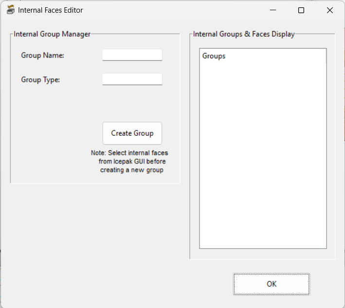
Internal Faces Editor
In the Internal Faces Editor, use the Internal Group Manager to manually create groups of internal faces based on geometry selected from the 3D Modeler window or the History tree.
| Internal Group Manager | ||
|---|---|---|
| Group Name |
Enter a Group Name for the group of internal face geometry. |
|
|
Group Type |
Enter a Group Type for the group of internal face geometry. |
|
|
Create Group |
Click Create Group to save the group name and/or type changes. The Create Group button appears when a group is selected in the Groups tree. |
|
| External Groups & Faces Display | ||
| Group Tree | The Internal Groups & Faces Display tree lists the groups and associated faces you've created. If needed, select a group and modify its name or type. From a group's right-click menu, you can unite all the faces into one piece of geometry, delete the group, or delete all groups. From an internal face's right-click menu, you can split the face, remove it, or move it to a different group. With multiple faces selected, you can split the faces, unite them, remove them, or move them to a different group. | |
| OK | After creating all internal groups, click OK to save the internal groups and close the Internal Faces Editor dialog box. | |
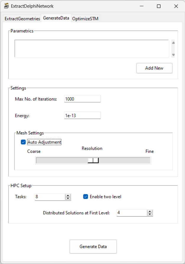
Generate Data Tab
The Generate Data tab controls the creation, analysis, and post-processing of parametric variations. Boundary conditions, including source powers and ambient temperature, as well as monitor points are generated. It also contains settings for simulation iterations, energy convergence, mesh, and high performance computing. The solutions extracted from the solved parametrics can then be used as training and/or test data sets on the Optimize STM tab.
|
Parametrics |
||
|---|---|---|
|
Add New |
Under Parametrics, click Add New to open the New Parametric Setup Editor dialog box. See New Parametric Setup Editor for information on specifying parametric setup settings. From a setup's right-click menu, you can change the solution type, delete it, create the parametric setup under Optimetrics in the Project Manager, or initiate post-processing of a setup that was analyzed individually. |
|
| Note: If you add multiple setups, you can use the right-click options to create and post-process them individually instead of clicking Generate Data, which creates, analyzes, and post-processes all setups in the Parametric field. Analyzing the parametric setups individually from the Project Manager also allows you to optimize your High Performance Computing settings for complex models. | ||
|
Settings |
||
| Max No. of Iterations | Max No. of Iterations specifies the maximum number of solution iterations to be performed in a simulation. | |
| Energy | Energy specifies the convergence criterion for the parametric trials. When the residual is less than or equal to the specified value, the solution will be considered converged. | |
| Transient Settings | Click Transient Settings to open the Transient Settings Editor dialog box. See The Icepak Solve Setup Dialog (Transient) for more information on transient settings. The Transient Settings button is only available when one or more parametric setups in the list has a transient solution type. | |
| Mesh Settings | Select Auto Adjustment to display the automatic mesh settings slider bar. The slider bar is a visual representation of the resolution you choose as ranging from coarse resolution with a small mesh size through a five-position scale to a fine resolution with a large mesh size. See Defining Global Mesh Settings for more information on automatic mesh settings. | |
|
HPC Setup |
||
| Tasks | Under HPC Setup, specify the high performance computing settings. For more information on tasks and two-level job distribution, see High Performance Computing in Icepak. | |
| Enable two level | ||
| Distributed Solutions at First Level | ||
|
|
||
|
Generate Data |
Click Generate Data to begin solving the parametric setups listed in the Parametrics field. |
|
New Parametric Setup Editor
The New Parametric Setup Editor allows you to configure and add parametric setups to add to the Parametrics field on the Generate Data tab. Configure parametric setups based on three approaches:
Predefined
The Predefined approach loads a parametric setup containing default parametric variations.
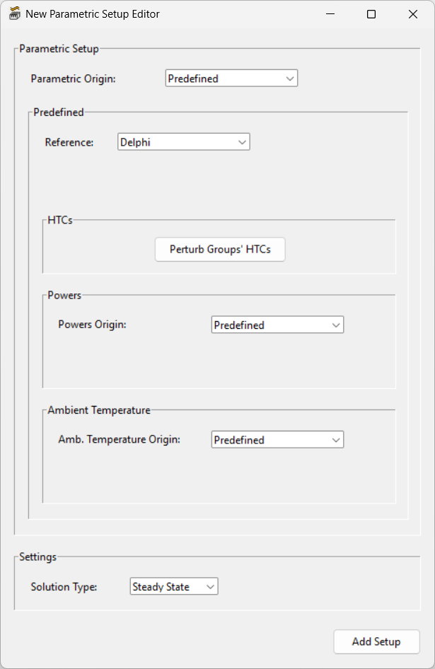
| Parametric Setup - Predefined Origin | ||
|---|---|---|
| Predefined | ||
| Reference | Select the variation set for the parametric trials. Delphi uses the set used for training by the Extract Delphi Network toolkit in Electronics Desktop version 2023 R2. JEDEC uses the set used for validation by the Extract Delphi Network toolkit in Electronics Desktop version 2023 R2 and defined by the JESD15-4 DELPHI model guidelines. Demo uses a set of seven variations for fast data generation. | |
| HTCs | ||
| Perturb Groups' HTCs | Click Perturb of Groups' HTCs to open the Perturbation Editor for Groups' HTCs dialog box. Enter a standard deviation for the perturbation of each external face group. | |
|
Note: The heat transfer coefficient for each external face is obtained by multiplying the associated groups' heat transfer coefficient by a multiplicative perturbation obtained by sampling a normal distribution characterized by mean = 1 and standard deviation = the specified value. A standard deviation equal to 0.0 corresponds to no perturbation around the group's value. |
||
| Powers | ||
| Power Origin | By default, Predefined is selected to use the default power values for the parametric trials. If needed, click Edit Ranges to specify a range of power in the Power Ranges Editor dialog box. | |
| Ambient Temperature | ||
| Amb. Temperature Origin | By default, Predefined is selected to use the default ambient temperature values for the parametric trials. Alternatively, select Uniform Sampling and enter minimum and maximum values for the range of ambient temperatures. | |
| Settings | ||
| Solution Type | Select Steady State or Transient to set the solution type. | |
| Add Setup | Click Add Setup to create the parametric setup and add it to the Parametric field on the Generate Data tab. | |
Sample
The Sample approach generates new parametric variations based on a specified sampling method.
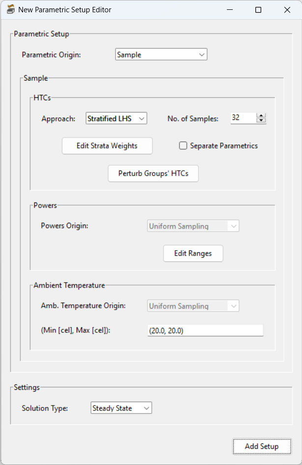
| Parametric Setup - Sample Origin | ||
|---|---|---|
| Sample | ||
| Approach | Approach specifies the method for sampling in the hyper-space of heat transfer coefficients for the parametric trials. Stratified LHS specifies Stratified Latin Hypercube Sampling. A hyper-space of heat transfer coefficients is defined for the  -th physical environment, and -th physical environment, and  variations are sampled from it based on Latin Hypercube Sampling (Note: variations are sampled from it based on Latin Hypercube Sampling (Note:  ). See Stratified LHS for more information. LHS specifies Latin Hypercube Sampling. Uniform specifies a sample set that is divided equally within the range. ). See Stratified LHS for more information. LHS specifies Latin Hypercube Sampling. Uniform specifies a sample set that is divided equally within the range. |
|
| No. of Samples | Specify the number of samples to include in the variation set. | |
| Edit Strata Weights | For Stratified LHS, click Edit Strata Weights to open the Stratified LHS dialog box. Specify the percentage of variations to be sampled in each environment. See Stratified LHS for more information on strata weights. | |
| Separate Parametrics | For Stratified LHS, select Separate Parametrics if a separate parametric study is needed for each of the environments. | |
| Perturb Groups' HTCs | Click Perturb of Groups' HTCs to open the Perturbation Editor for Groups' HTCs dialog box. Enter a standard deviation for the perturbation of each external face group. | |
| Note: The heat transfer coefficient for each external face is obtained by multiplying the associated groups' heat transfer coefficient by a multiplicative perturbation obtained by sampling a normal distribution characterized by mean = 1 and standard deviation = the specified value. A standard deviation equal to 0.0 corresponds to no perturbation around the group's value. | ||
| Power | ||
| Power Origin | By default, Uniform Sampling is selected to specify random variations of power values for the parametric trials. If needed, click Edit Ranges to specify a range of power in the Power Ranges Editor dialog box. | |
| Ambient Temperature | ||
| Amb. Temperature Origin | By default, Uniform Sampling is selected to specify random variations of ambient temperature values for the parametric trials. Alternatively, select Uniform Sampling and enter minimum and maximum values for the range of ambient temperatures. | |
| Settings | ||
| Solution Type | Select Steady State or Transient to set the solution type. | |
| Add Setup | Click Add Setup to create the parametric setup and add it to the Parametric field on the Generate Data tab. | |
Stratified LHS
Stratified LHS uses stratified sampling to divide a population into distinct groups, or “strata,” so that each group is homogeneous in some respect. In this case, each stratum represents a different physical environment. Once the population is divided into strata, a random sample is then drawn from each stratum based on Latin Hypercube Sampling.
You can specify strata weight in the Stratified LHS dialog box. Enter weight values for each physical environment, including forced convection, free convection, heat sink, cold plate, and fluid bath.
You can select Bottom and/or Top for Forced Convection, Heat Sink, and Cold Plate to specify that the conditions be applied to the bottom and/or top faces, respectively.
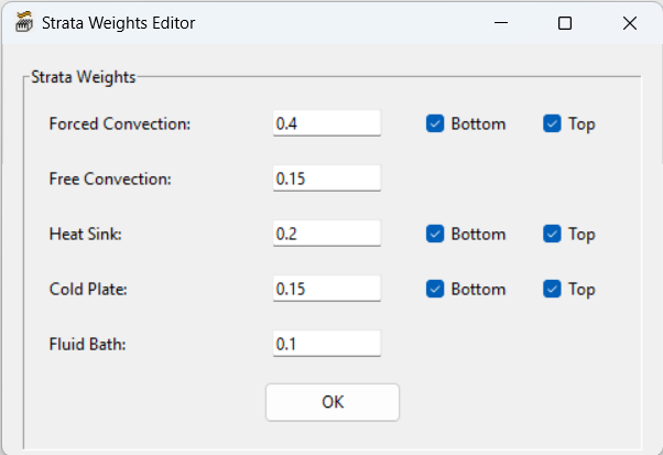
This approach ensures that ensures no variations are sampled in unphysical heat transfer coefficient regions and each stratum is properly represented in the parametric setup based on the importance designated by the strata weights. This potentially increases the representation and accuracy of the overall sample compared to simple random sampling.
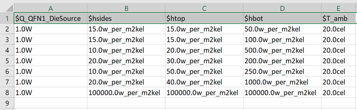
Import from File
Import from File allows you to generate parametric trials specified in a comma-separated value (.csv) file. Each column in the file must have a header column that includes the variable name with the cells beneath it listing the values. Each value cell must include a unit of measure.
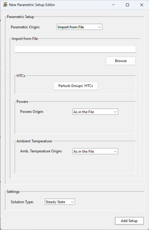
| Parametric Setup - Import from File Origin | ||
|---|---|---|
| Import from File | ||
| Browse | Click Browse to navigate to search for and select the .csv file. | |
| HTCs | ||
| Perturb Groups' HTCs | Click Perturb of Groups' HTCs to open the Perturbation Editor for Groups' HTCs dialog box. Enter a standard deviation for the perturbation of each external face group. | |
|
Note: The heat transfer coefficient for each external face is obtained by multiplying the associated groups' heat transfer coefficient by a multiplicative perturbation obtained by sampling a normal distribution characterized by mean = 1 and standard deviation = the specified value. A standard deviation equal to 0.0 corresponds to no perturbation around the group's value. |
||
| Powers | ||
| Power Origin | By default, As in the File is selected to specify the power values defined in the .csv file. Alternatively, select Uniform Sampling and Click Edit Ranges to replace all the power values with samples from uniform distributions in the range specified in the Power Ranges Editor dialog box. | |
| Ambient Temperature | ||
| Amb. Temperature Origin | By default, As in the File is selected to specify the ambient temperature values defined in the .csv file. Alternatively, select Uniform Sampling to replace all the ambient temperature values with samples from a uniform distribution in a specified range. | |
| Settings | ||
| Solution Type | Select Steady State or Transient to set the solution type. | |
| Add Setup | Click Add Setup to create the parametric setup and add it to the Parametric field on the Generate Data tab. | |
The following image displays an example of the acceptable format of a .csv file.
Optimize STM Tab
The Optimize STM tab controls the construction, training, and export of the Delphi-like Surrogate Thermal Model (STM), starting from DTM (Detailed Thermal Model) data produced in the previous tab or coming from external sources.

| Data Files | ||
|---|---|---|
| Training | Click Add File and select the parametric trial data for the optimizer to use for training. | |
| Testing | Click Add File and select the parametric trial data to use for testing against the results of the optimizer. | |
| Note: The training and testing data is saved comma-separated value (.csv) files appended with "_monitors" (steady-state) or "_aedtexport" (transient) at the end of the file name. | ||
| Graph Nodes | ||
| Real Nodes Settings | Click External and/or Internal to open the Node Selection dialog box. See Node Selection for more information about selecting an approach to modeling network nodes. | |
| No. of Fict. Internal Nodes | Specify the number of fictitious internal nodes to include in the network. Fictitious nodes do not correspond to any sources, external faces, or other real parts of the package. They are added to the graph only to increase its predictive capacity, and they are connected to all other nodes in the network. | |
| No. of Intermediate Nodes | For transient simulations, specify the number of intermediate nodes. Intermediate nodes are fictitious internal nodes that are placed on a network schematic edge to split this into multiple sub-edges. They are added to the network schematic only to increase its predictive capacity, and they are only connected to two other nodes. | |
| Equally Dist. Intermediate Nodes | For transient simulations, adjust the slider bar to control the distribution of the intermediate nodes on the network schematic. The right extreme of the bar distributes intermediate nodes on the schematic as equally as possible (i.e., all the network schematic edges will be split into the same number of sub-edges). The left extreme of the bar assigns intermediate nodes to the edges characterized by smaller thermal resistances (i.e., by preferential heat-pathways). | |
| Note: Capacitances are assigned to dinternal nodes, including sources and fictitious and intermediate nodes (if any). | ||
| Parameters Initialization | ||
| Add File | For transient simulations, click Add File and select the yinf.csv file, which contains thermal conductance data from a previous steady-state training to improve the steady-state behavior of the CTM. If needed, right-click the file and select Fix During Optimization to ensure the thermal resistance values are fixed to the ones learned from steady-state simulations and not retrained and updated. | |
| Note: In order to use the previously generated thermal conductance data, the steady-state component of the DELPHI network schematic must be identical to the previous schematic (i.e., the settings for external nodes and fictitious internal nodes must be identical to the ones previously used for steady-state training). | ||
| Optimizer | ||
| Algorithm | Select the Gradient-Based or Differential Evolutionary to specify the algorithm used to train the data. See Gradient-Based Settings and Differential Evolutionary Settings for a list of their respective settings. | |
| Settings | Click Settings to open the Gradient-Based Algorithm or Differential Evolutionary Algorithm dialog box and define the settings for the training. | |
| Optimize STM | Click Optimize STM to begin training the STM. | |
| Query STM | Click Query STM to open the STM Querying Settings dialog box. Select the STM file , a Querying Mode, and a data file generated by the optimetrics trials. In the Delphi-like S.T.M. Predictions - From Data File dialog box, compare the DTM to the STM. Select Int. Features to view the temperature data on the real internal nodes. | |
| Export STM | Click Export STM to generate an Electronics Desktop 3D component (.a3Dcomp) file, which is saved in a new folder in the project directory (prepended with "Train_"). Results images are also located in this directory. | |
Node Selection
In the Node Selection dialog box, define the approach for creating network nodes for each group of external faces.

| Groups | ||
|---|---|---|
| Groups | Groups lists the groups of external faces. Select a group from the groups list to define its Approach Settings. | |
| Approach Settings | ||
| Group | Group displays the selected group. | |
| Approach | From the Approach drop-down list, select Automatic, Group-Specific, or Face-Specific. Automatic maps two or more faces in the group to a node if their temperature difference is below specified thresholds. Group-Specific creates one node for the entire group of faces. Face-specific creates a node for each face in the group. | |
Note: The  -th face contributes to the corresponding -th face contributes to the corresponding  -th group's node with weight -th group's node with weight  . .
|
||
| Mean Relative Difference [%] | For the Group-Specific, define the mean and max relative temperature difference for the creation of network nodes. | |
| Max Relative Difference [%] | ||
Gradient-Based Algorithm Settings

Differential Evolutionary Algorithm Settings

Training Results
In the training files directory, open the .png image file appended with "_error_bars" to view the temperature mean and max temperature error percentage.