Editing Distributed Machine Configurations for Icepak

To create a new distributed machine configuration, or edit an existing machine configuration.

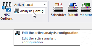
1. Click Tools > Edit Active Analysis Configuration to open the Analysis Configuration dialog directly or click Analysis Config on the Simulation tab of the ribbon toolbar.


This opens the Analysis Configuration dialog box directly. You can also access this dialog from the HPC and Analysis Options dialog box by clicking the Add..., Edit..., or Copy... buttons.

If you have selected Add... from the HPC and Analysis Options dialog box, the fields are empty. If you have selected Edit..., used Tools > Edit Active Analysis Configuration, or clicked Copy from the HPC and Analysis Options dialog box, the fields show the selected configuration.


2. Specify the name of the new or edited configuration. It cannot be empty and cannot be a previously used name or a reserved word.
3. Optionally, click Use Automatic Settings. The Job distribution tab and Tasks column are no longer available.

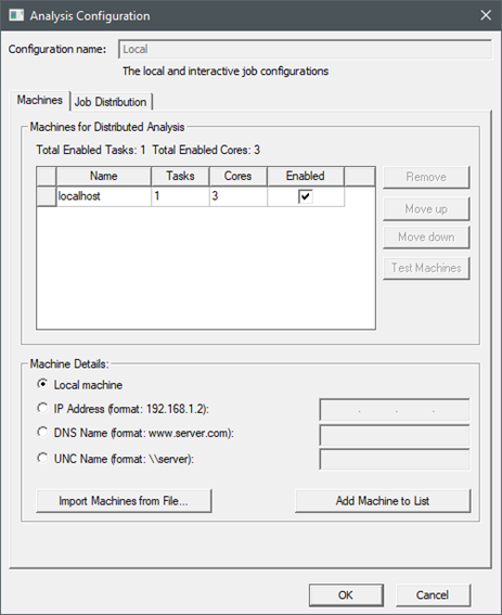
Machines Tab

This tab contains the machine list for the analysis configuration. Here you can provide machine information, either by specifying Remote machine details, or by importing a list of machines from a file. You can then remove, order, test, and enable machines on the list. Control buttons let you Add machine(s) to list or Remove machines from the list.

Import Machines from File...

You can import a machine list from a file, and an enhanced the file format handles the new flexibility. Each line of the file can contain a machine specifier of the form:

<MachineName>:<NumTasks>:<NumCores>.

Note:

This same format is used with the "-machinelist file=" command line option.

Local Machine Radio Button

To streamline the common case of running jobs on the current machine, use the dedicated radio button to specify the local machine.

4. For each machine to manually add to the list, under Machine Details, specify an IP address, a DNS name, or a UNC name. Then, click Add Machine to List.

The remote machines must have the same Ansys Electromagnetics Suite version installed in the same OS and version, and have the RSM service active.

Once you have specified the remote machine details, either directly or by Importing Machine from a File, you select a machine from the table to enable the buttons to Remove a machine, or to Move a machine up or down on the list.



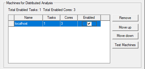
The displayed list always shows the order in which you entered them irrespective of the load on the machines. To control the list order, select one or more machines, and use the Move up or Move down buttons. Move up and Move down are enabled when you select one or more adjacent machine names.

Enabled Machines

Each machine on the current list has an Enabled check box. Here you can enable or disable the listed machines according to circumstance. Above the table, the dialog gives a count of the total enabled tasks, and the total enabled cores.

Note:
• Icepak uses the Tasks setting to control the number of concurrent meshing processes for handling multiple mesh regions. For single-level job distuibutions, when Optimetrics is enabled under the Job Distribution tab, the number of Optimetrics variations to solve in parallel is also controlled by this settting.
• The Cores setting is used by the solver only during the mesh processing stage. Note that, during the solution iterations stage, the Icepak solver automatically chooses the number of cores to balance the computational resources on the machine. The Cores setting has no effect on this allocation.
• The number of cores you specify must be equal to or greater than the number of tasks you specify.

For distributed tasks in Icepak, the software will allocate the cores on a given machine to that machine's tasks. For example, if you want to solve 5 Optimetrics variations, each being allocated 2 cores, you must specify 5 tasks and 10 cores. The software will automatically allocate 2 cores to each of the 5 variations.

Consider a given set of variations (for example, different thermal properties or object dimensions). Ideally, you would make assignments so that each task has the same number of cores. This is because the solvers attempt to make each task computationally balanced for the greatest solution efficiency. For example, consider two machines, one with eight cores, and another with four. Assuming that the memory is proportionally equivalent, you could assign 2 tasks to machine 1 and assign 1 task to machine 2, giving all tasks the same number of cores (4).

If you select a distributed configuration (rather than Local) from the Toolbar menu and you launch multiple analyses from the same UI. Icepak selects the machines that are running the fewest number of engines in the order in which the machines appear in the list. For example, if the list contains 4 machines, and you launch a simulation that requires one machine, Icepak chooses the first machine in the list. If another simulation is launched while the previous one is running, and this simulation requires two machines, Icepak chooses machines 2 and 3 from the list. If the first simulation then terminates and we launch another simulation requiring three machines, Icepak chooses 1, 4, and 2 (in that order).

Test Machines

When multiple users on a network are using distributed solve or remote solve, they should check the status of their machines before launching a simulation to ensure no other Ansys EM processes are running on the machine. To do this, you can select one or more machines and click Test Machines. A Test Machines dialog box opens.

The test goes through the current machine list and gives a report on the status of each machine. A progress bar shows how far testing has gone. An Abort button lets you cancel a test. When the test is complete, you can OK to close the dialog box. If you need to disable or Enable machines from the list based on the report, you can do so in the Distributed Analysis Machines dialog box.

Job Distribution Tab

Use this tab to enable specific types of job distribution and to enable multi-level solves. The Job distribution types listed are design type specific and will differ between products.

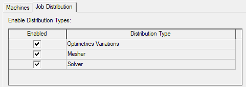
Use the check boxes to enable/disable available distribution types. The job distribution list box allows you to specify which job distribution types to allow for the current analysis configuration. At solve time, the Ansys Electronics Desktop automatically select the best distribution type from the enabled distribution types. By enabling/disabling distribution types, you can control the job distribution.

When using job distribution for meshing, you must specify the optimal number of Tasks on the Machines tab. The number of tasks required is the number of mesh regions (including the global mesh region) plus one task for the mesh controller. For example, if you've created three mesh regions in your model, specify at least five tasks: three for the mesh regions, one for the global mesh region, and one for the mesh controller. For this example, if you specify more than five tasks, the Electronics Desktop ignores the extra tasks. Conversely, if you specify fewer than five tasks, one or more mesh regions are meshed serially rather than concurrently.

Just because you enable a distribution type does not mean it will be used. It must be also allowed by the solve setup. Note that the enabled distribution types will apply to all setups of the given design type, so it is possible for different setups in a design to be solved using different distribution types.

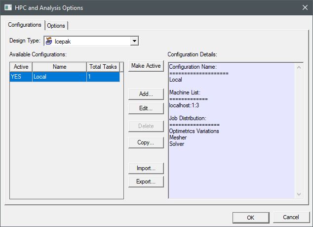
The distribution types that you enable here are listed in the HPC and Analysis Options dialog box in the Configuration Details section. To access this dialog box, click Tools > Options > HPC and Analysis Options from the menu bar or click the HPC and Analysis Options command on the Simulation ribbon tab.

For products that support two-level distribution, when the design is appropriate, you can turn on two level distributed solutions, and specify the number of engines to use for level 1. An example design that could use two level distribution would be an array with frequency sweeps.

Distribution Levels (for Icepak)

The radio buttons let you enable/disable two level distribution.

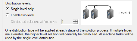
If you select single level, one distribution type will be applied at each stage of the solution process. If multiple types are available, the higher level solution will generally be distributed. All machine tasks will be used by the single-level distribution.

Selecting Enable two level enables the Distributed Solutions at first level selection box.

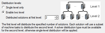
If you select Enable two level, the first level will distribute the specified number of solutions. Each solution will use a subset of machine tasks to distribute the second level. A solver distribution type must be available for the second level, otherwise single-level distribution will be applied.

The Preview Job Distribution Setup menu and field lets you view how the selected setup will be distributed.

Distributed Solutions at First Level 1

This control determines how many level 1 tasks to create during a two level distribution. This indirectly determines how many level 2 tasks for each level 1 task are used: the total number of tasks is specified by the list of enabled machines on the first tab, and the software evenly distributes resources among the L1 tasks which then are used to spawn off level 2 tasks.

Example:

• You create a machine list with 20 enabled tasks.
• You enable Variations and Solver.
• You enable 2 level distribution with distributed solutions at first level = 3.
• You solve a parametric analysis.

For the parametric analysis, the level 1 distribution type is Variations and the level 2 distribution type is Solver. Since the number of level 1 tasks = 3, three variations are launched simultaneously. The number of enabled tasks is 20. Those 20 tasks will be split as evenly as possible over the 3 variations. For the solver, Variations 1 & 2 will each get 7 tasks (processes) and Variation 3 will get 6 tasks (processes) to use for Solver distribution.

Adding Configurations or Accepting Edits

Click OK to accept the changes and close the Analysis Configuration dialog box. Only machines checked as Enabled appear on the distributed machines Configuration Details Machine list.

Regardless of the machine(s) on which the analysis is actually run, the number of processors and the default process priority settings are now read from the machine from which you launch the analysis. See Setting HPC and Analysis Options.

For more information, see distributed analysis.