
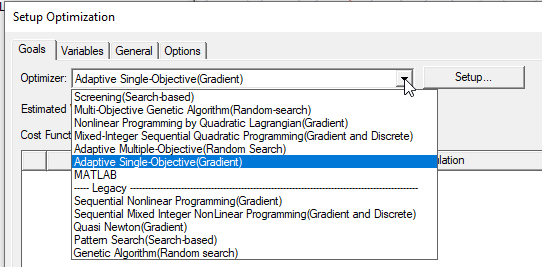
Choosing an Optimizer
Conducting an optimization analysis allows you to determine an optimum solution for your problem. In optimization analyses, there are many available optimizers.
Goal Driven Optimizers
These use a Decision Support Process (DSP) based on satisfying criteria as applied to the parameter attributes using a weighted aggregate method. In effect, the DSP can be viewed as a post-processing action on the Pareto fronts as generated from the results of the various optimization methods.
- Screening (Search based) – a non-iterative direct sampling method that uses a quasi-random number generator based on the Hammersley algorithm. You can start with Screening to locate the multiple tentative optima and then refine with NLPQL or MISQP to zoom in on the individual local maximum or minimum value. Usually Screening is used for preliminary design, which can lead you to apply one of the other approaches for more refined optimization results.
- Multi-Objective Genetic Algorithm – an iterative random search algorithm that can optimize problems with continuous input parameters. It is better for calculating the global optima. You can start with MOGA to locate the multiple tentative optima and then refine with NLPQL or MISQP to zoom in on the individual local maximum or minimum value.
- Nonliner Programming by Quadratic Lagrangian (Gradient) – a gradient-based, single-objective optimizer based on quasi-Newton methods. Ideally suited for local optimization.
- Mixed-Integer Sequential Quadratic Programming (Gradient and Discrete) – a gradient-based, single-objective optimizer that solves mixed-integer non-linear programming problems by a modified sequential quadratic programming (SQP) method. Ideally suited for local optimization.
- Adaptive Multiple Objective – an iterative, multi-objective optimizer that employs a Kriging response surface and MOGA. In this method, the use of a Kriging response surface allows for a more rapid optimization process because all design points are not evaluated except when necessary and part of the population is simulated by evaluations of the Kriging response surface, which is constructed of all design points submitted by Multi-Objective Genetic Algorithm (MOGA).
- Adaptive Single Objective (Gradient) – a gradient-based, single-objective optimizer that employs an OSF (Optimal Space-Filling) DOE, a Kriging response surface, and MISQP.
- MATLAB
All optimizers assume that the nominal problem you are analyzing is close to the optimal solution; therefore, you must specify a domain that contains the region in which you expect to reach the optimum value.
All optimizers allow you to define a maximum limit to the number of iterations to be executed. This prevents you from consuming your remaining computing resources and allows you to analyze the obtained solutions. From this reduced range, you can further narrow the domain of the problem and regenerate the solutions.
All optimizers also allow you to enter a coefficient in the Add Constraints window to define the linear relationship between the selected variables and the entered constraint value. For the SNLP and SMINLP optimizers, the relationship can be linear or nonlinear. For the Quasi Newton and Pattern Search optimizers, the relationship must be linear.
Cost functions can be quite nonlinear. As a result, during the function evaluations of the algorithm, the cost function can vary significantly. Also, it is important to understand the relationship between optimization function evaluation and iteration. Every iteration, depending on the number of parameters to be optimized, performs several function evaluations. These function evaluations, depending on how nonlinear the cost function is, could show drastic changes. The presence of drastic changes has no bearing on whether the optimization algorithm converged or not.
In the case of non-gradient search-based optimization algorithms, such as "pattern search," which are entirely based on function evaluations, one could see drastic changes in the function evaluations depending on how nonlinear the cost function is. This could seem misleading as if the algorithm did not converge since in theory one expects the cost function to decrease from one iteration to the next. The optimetrics, however, reports function evaluations and not necessarily the optimizer performance per iteration.
The MATLAB optimizer displays function evaluation when the Show all functions evaluation check box is selected. If the check box is not selected, it displays iteration.
Legacy Optimizers
These include: