


To model sliding contacts in implicit analyses, use Mortar contacts [6]. Mortar contacts are segment-based using a penalty formulation and allow for finite sliding in each implicit time step. They are a very general type of contact that can handle edge-to-edge contacts for shells and solids plus contact situations involving beam elements and element erosion.
The input syntax for Mortar contacts was slightly changed from R10 of LS-DYNA, see
Mortar Contacts in R9 and Earlier. Not all features of Mortar contacts are
presented here. For a complete description of the present features of Mortar contacts,
see the general remarks section of the *CONTACT keyword in Keyword Manual Vol. I .
Ansys recommends that you define the sliding contacts based on parts or part sets. For surfaces involving higher order elements, part or part sets must be used in the contact definitions.
Ansys recommends using the contact type *CONTACT_AUTOMATIC_SURFACE_TO_SURFACE_MORTAR_ID in situations where contacts can be defined pairwise in a convenient way between two obvious surfaces, and self-contact need not be considered [6]. Ansys also recommends using the "softer" (less stiff material or coarser mesh)
part as a tracked surface. A template for using the surface-to-surface Mortar contact (versions R10 and later) follows:
*CONTACT_AUTOMATIC_SURFACE_TO_SURFACE_MORTAR_ID
Define contact ID, Heading
Card 1: Define what shall be in contact using parts or part sets
Card 2: Define friction
Card 3: Define alternative penalty stiffness (SFSA)and thicknesses
                    (SAST) for shells, or leave blank to get defaults
Card 4: blank / optional
Card 5: Define contact thickness for solids (PENMAX)or leave blank
Card 6: optional / Define IGAP and IGNORE
Cards 1 - 3 must be defined. Cards 4 - 6 are optional.
Using the PENMAX Parameter to Specify Contact Thickness
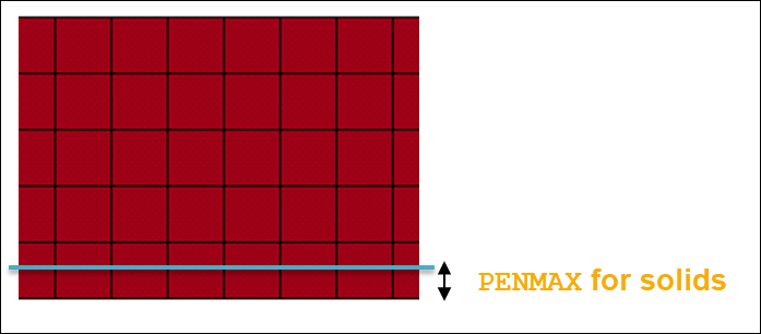
If solid elements are involved in the contacts, you can specify their contact thickness by using the PENMAX parameter on Optional card B (Card 5). (In versions prior to R10, the contact thickness for solids was defined by the SAST parameter, see Mortar Contacts in R9 and Earlier) The contact thickness for solids can be seen as the thickness of the zone below the surface of the solid part, where the penalty forces will be applied to push out penetrating nodes. This is shown in Figure 6.1: Using PENMAX to define the contact thickness for solid parts..
Figure 6.2: Mortar penalty force as a function of penetration (schematic). shows how this distance is related to relative penetration distance, which is used for calculating the penalty force. By reducing PENMAX, a stiffer contact (for solid parts) can be obtained, but at the same time the risk that a tracked segment will be released from the contact increases. It is important to note that the PENMAX parameter for solids specifies a physical distance, which means that the value must be reasonable with respect to the mesh size, as well as to the physical dimension of the involved parts.
If PENMAX is left blank, LS-DYNA automatically calculates a value for the contact thickness for solids. This works well in most cases, provided that the mesh in the contact surfaces is reasonably regular.
The Mortar contact uses a penalty formulation. This means that there will always be small penetrations between parts in contact. The penetration is required in order to transfer a contact force. The Mortar contact will report both relative as well as absolute values of the maximum penetrations during the simulation in the mes0* files before each implicit step begins, for example:
Contact sliding interface 1010
Number of contact pairs 2784
Maximum penetration is 0.1122220E-02 between
elements 14606 and 10263 on this processor
Maximum relative penetration is 0.9978402E-01 % between
elements 14606 and 10263 on this processor
Based on this example, you can judge what is acceptable in terms of penetration distance.
Specifying Contact Stiffness with the SFSA and IGAP Parameters
To reduce penetrations (if required), the contact stiffness can be increased by the two parameters: SFSA and IGAP, as shown in the following figure.
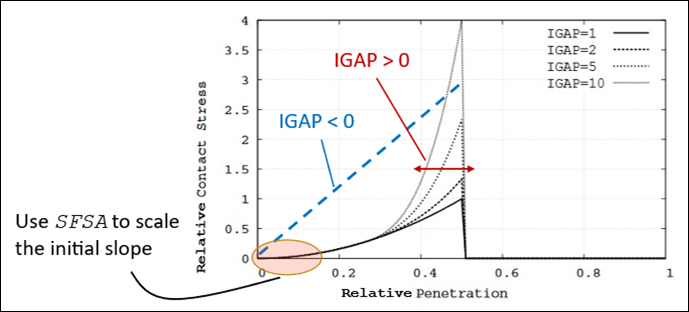
The stiffness scale factor SFSA controls the initial slope of the contact stiffness and can effectively be increased in order to reduce penetrations. The parameter IGAP controls the ramp-up of the penalty stiffness. It can be increased to reduce the risk of contacts being released. From R14 of the Ansys LS-DYNA software, the option IGAP < 0 switches to a linear relationship between the penetration and contact pressure. This can be helpful when relatively large penetrations are observed for small contact pressures. In most cases, modifying the default contact stiffness settings is not necessary.
Specifying Initial Penetrations with the IGNORE Parameter
The IGNORE parameter can be used to allow initial penetrations. (Within reasonable limits: Ansys recommends using the capabilities of your preferred preprocessing tool to check for and fix unintended initial contact penetrations.) For two parts with initial penetrations, the option IGNORE = 1 will track the penetrations. If the parts are separated and put into contact again, the first contact will occur at the physical surface of the parts, as shown in the following figure.
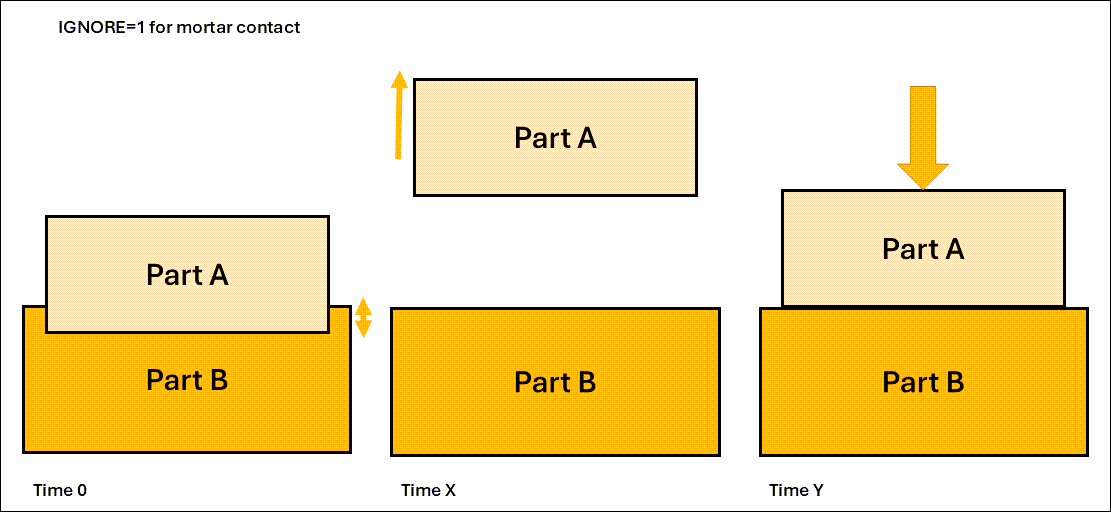
Parts A and B are initially penetrating at Time 0. At Time X, the parts are separated, for example by prescribed displacements. At Time Y, the parts are brought back into contact. Contact then occurs at the physical surface of the parts.
The option IGNORE = 2 (which is the default behavior) means that the contact surface is moved, so that when the parts come into contact again, it will be at the original position, as seen in the following figure.
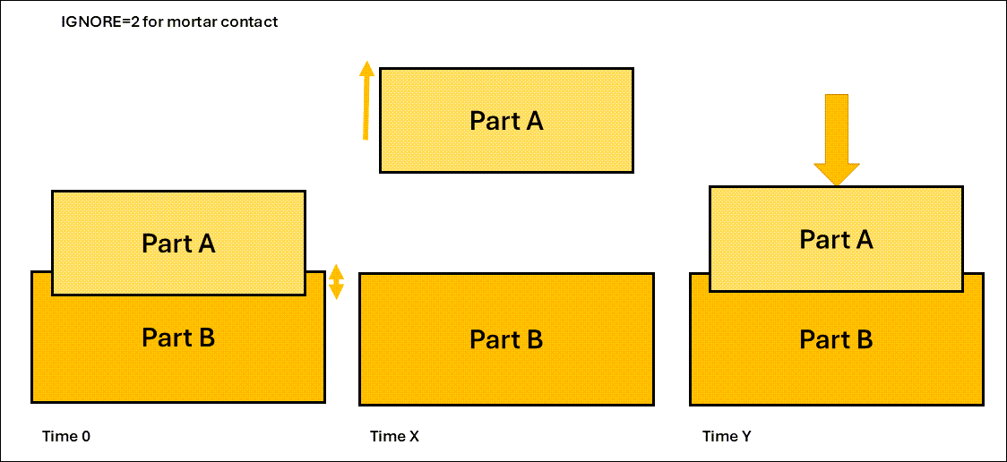
Parts A and B are initially penetrating at Time 0. At Time X, the parts are separated, for example by prescribed displacements. At Time Y, the parts are brought back into contact. Contact then occurs at the original intersecting surface of the parts.
The options IGNORE = 3, 4 can be used for resolving initial interferences, such as in a press-fit situation. The penetrations will then be resolved linearly between t = 0 and t = MPAR1, as specified on Card 6 of the contact card.
The option IGNORE = 3 is useful for initial penetrations that are small enough to be detected by the contact algorithm. For larger penetrations, the option IGNORE = 4 can be used, in combination with a user-specified search distance (MPAR2 on Card 6), which shall be at least as large as, and on the order of, the maximum initial penetration.
The use of IGNORE = 4 for resolving a press-fit between a rubber sleeve and a (rigid) steel housing is illustrated in the example Insert_and_interference.key.
For situations where self-contact must be considered or a single contact
definition is desired, Ansys recommends using
*CONTACT_AUTOMATIC_SINGLE_SURFACE_MORTAR_ID.
A template for using the automatic single-surface Mortar contact follows:
*CONTACT_AUTOMATIC_SINGLE_SURFACE_MORTAR_ID
Define contact ID, Heading
Card 1: Define what shall be in contact (only SURFA) by part or part set
Card 2: Define friction
Card 3: Define alternative penalty stiffness (SFSA)and thicknesses (SAST)
          for shells, or leave blank to get defaults
Card 4: blank / optional
Card 5: Define contact thickness for solids (PENMAX)or leave blank
Card 6: optional / Define IGAP and IGNORE
For the single-surface Mortar contact option, you can specify a version that ignores possible self-contact within the same part by setting IGNORE < 0. For example, setting IGNORE = -2 will have the same meaning as IGNORE = 2, but contacts between segments in the same part are ignored.
In general, Ansys does not recommended using contact damping in implicit analyses. For Mortar contacts, the contact damping settings will be ignored in an implicit static analysis.
From R10 (rev. 118243) of LS-DYNA, the input for the Mortar contact was modified. In versions prior to R10, the contact thickness for solids (compare Figure 6.1: Using PENMAX to define the contact thickness for solid parts.) was defined using the SAST parameter on Card 3. From version R10 onward, the contact thickness is defined by the PENMAX parameter as described in Surface-to-surface Contact.)
A template for using the Mortar surface-to-surface contact in LS-DYNA versions prior to R10 follows:
*CONTACT_AUTOMATIC_SURFACE_TO_SURFACE_MORTAR_ID
Define contact ID, Heading
Card 1: Define what shall be in contact using parts or part sets
Card 2: Define friction
Card 3: Define alternative penalty stiffness (SFSA, SFM) and thicknesses
                    (SAST) or leave blank to get defaults
Card 4: blank / optional
Card 5: blank / optional
Card 6: optional / Define IGAP and IGNORE (MPAR1, MPAR2)
Note: In versions prior to R10, when shells and solids are treated by the same single-surface Mortar contact, you cannot use the SAST parameter to specify a contact thickness for the solids. SAST is also used as the contact thickness for the shells.
In some cases, it is desirable to use non-Mortar contacts. For example,
*CONTACT_SURFACE_TO_SURFACE_INTERFERENCE_ID can be useful in some
situations to resolve a press-fit.
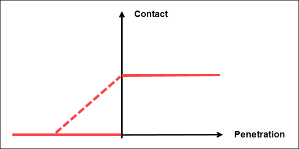
By default, a"sticky" behavior is active for all non-Mortar contacts. This means that contact forces are transferred before the surface gap is closed. Additionally, a certain amount of negative contact pressure can be transmitted between surfaces that are pulled apart again, as shown in Figure 6.5: Contact stiffness as a function of penetration for non-Mortar contacts.
This behavior is controlled by the IGAP parameter on Card 6 (optional card C) of the contact definition. In some situations, using sticky contact (IGAP = 1) can aid convergence. But in general, Ansys recommends turning it off (IGAP = 2). By setting IGAP > 2, the sticky contact is active for the first IGAP-2 iterations, and then turned off.
For non-Mortar contacts, a segment-based algorithm can be activated by setting SOFT = 2.
The following figure shows contact stiffness for non-Mortar contacts as a function of penetration for IGAP = 1 (dashed line) and IGAP = 2 (solid line).
The *RIGIDWALL option is a special case for sliding contacts. It
allows you to specify contact (including friction) with an analytical rigid surface.
This contact type is used in explicit (crash event) analysis.
Although there are situations where rigid walls work for implicit analysis, Ansys
generally recommends that you mesh the rigid wall as a normal part using
MAT_RIGID. Next, use a Mortar contact definition to impose the
desired contact condition.
For example, shell structures involving metallic materials can work reasonably
well with *RIGIDWALL in an implicit analysis. Plastic components meshed
with solid elements can end up with unrealistically large penetrations.
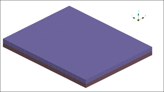
Non-Mortar sliding contacts will (in some cases) be linearized in eigenvalue analyses. If the contact surfaces initially are slightly over-closed or touch exactly, the surfaces may be tied in the normal direction. However, the surfaces are free to move relative to each other in the tangential direction. If the gap between the contact surfaces is initially open, no contact forces will be transferred. This case is shown in the following figure.
Figure 6.6: Contact surfaces that are touching (left) or have an initial gap (right)
 |
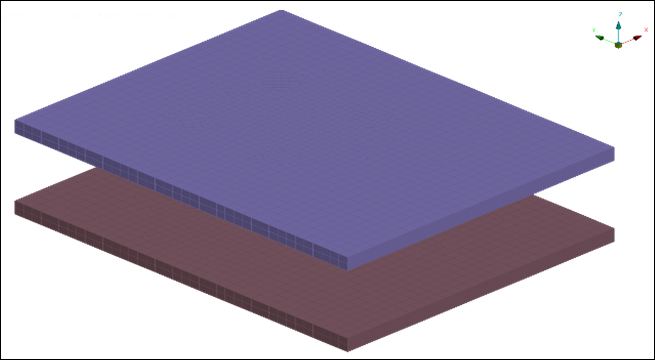 |
| Two contact surfaces that are initially touching. For this case, using non-Mortar contacts in a linear analysis, the surfaces may be tied in the normal direction but free to move in the tangential direction. | Two contact surfaces with an initial gap. For this case, no contact forces will be transferred in a linear analysis. |
The linearization procedure for non-Mortar contacts may lead to unintended overestimation of eigenvalues. For example, if a finite element (FE) mesh is taken from an automotive crash simulation model (where initial penetrations may exist) and non-Mortar contacts are used, the linearization may "tie" parts together. This in turn leads to unrealistically high eigenvalues.
In cases like this, be careful to introduce tied contacts only where you intended, in a way that you control. Some of the options for eigenvalue analyses are as follows:
If no additional tied contacts are intended, simply remove the non-Mortar contact definitions. Alternatively, replace them all with Mortar contacts.
If a behavior where parts appear as "glued" or "welded" together is desired, introduce tied contacts in the appropriate areas (see Tied Contacts).
If linearized contacts (where parts in contact are kept together but can slide against each other) are desired, start with a penetration-free model. Next, apply preloading (bolt pretension, gravity, and so forth) in a nonlinear step. Then, do an intermittent eigenvalue analysis (see Intermittent Eigenfrequency Analysis of a Bolted L-bracket).
Mortar sliding contacts do not transfer forces in eigenvalue analyses unless pre-loading is introduced by a preceding nonlinear case.
Sliding contacts will be appropriately linearized during intermittent eigenvalue analyses and intermittent linear buckling analyses (for example, if activated by pre-loading), see Intermittent Eigenfrequency Analysis of a Bolted L-bracket. This means that surfaces that come into contact during the pre-loading and have a contact pressure acting on them will appear in the eigenvalue analysis to be connected by stiff springs (from the contact stiffness) in the normal direction while being able to slide in the tangential direction (depending on the coefficient of friction). No new contacts can occur during the eigenvalue analysis and the ones detected during the nonlinear preload cannot be removed or unloaded.
Contact forces are also computed and output in linear transient modal dynamic analyses (see Contact Output), but are not applied to the structure. This lets you use the contact force as an indicator of initially open contact gaps closing during the simulation.
In linear static analyses (nsolvr = ±1 on *CONTROL_IMPLICIT_SOLUTION, as described in Linear Static Analysis) the use of sliding contacts is not recommended. Sliding contacts are nonlinear interactions that are incompatible with a purely linear analysis. The contact forces are computed and applied to the structure. But
since no equilibrium iterations are performed, the results will make little sense. These contacts may appear to be tied in linear analyses due to the "sticky" option (IGAP = 1 of non-Mortar contacts, see Non-Mortar Contacts, SOFT, IGAP and
Sticky Contact). If such behavior is desired, Ansys recommends that you replace the non-Mortar contacts with proper tied
contacts.
To include heat transfer by contacts and gap radiation in thermal or coupled
thermal structural analysis, use
*CONTACT_AUTOMATIC_SURFACE_TO_SURFACE_MORTAR_THERMAL_ID. The
thermal contacts also account for heat generated by friction. See Output From Thermal Analyses for an example of a coupled thermal
mechanical analysis involving thermal contact.
A template for using the automatic surface-to-surface Mortar contact (versions R10 and later) with thermal options follows:
*CONTACT_AUTOMATIC_SURFACE_TO_SURFACE_MORTAR_THERMAL_ID
Define contact ID, Heading
Card 1: Define what shall be in contact using parts or part sets
Card 2: Define friction
Card 3: Define alternative penalty stiffness (SFSA)and thicknesses (SAST)
                    for shells, or leave blank to get defaults
Card 4: Define thermal contact properties (gap conductance, radiation factor etc.)
Card 5: Define contact thickness for solids (PENMAX)or leave blank
Card 6: optional / Define IGAP and IGNORE
In the following, the separation or gap in the contact is denoted as lgap. The parameters that can be defined are:
LMIN specifies the contact gap (lgap) for which the thermal contact is treated as closed. For lgap > LMAX the thermal contact is not active.
H0 is the heat transfer conductance for a closed contact gap, used for contact gaps in the range 0 less than or equal to lgap less than or equal to LMIN.
K, which can be used to model a fluid between the contact surfaces. Then K is the thermal conductivity of the fluid, and the conductance calculated by LS-DYNA will be hcond = K / lgap.
FRAD is the radiation factor between the contact surfaces. This can be used to model heat transfer due to radiation of surfaces close to each other. Based on the reference-side temperature Tm and the tracked-side temperature Ts, LS-DYNA will calculate a radiant heat transfer conductance as
 .
.FTOSLV - describes how to distribute the sliding friction energy between the tracked and reference surfaces.
In summary, the contact conductance h will be given by

See the THERMAL section of the *CONTACT keyword in
Keyword Manual Vol. I for more
details.
By setting the variable BC_FLG = 1, convection boundary
conditions (*BOUNDARY_CONVECTION) applied to a surface that is also
involved in a thermal contact will be de-activated for the segments where the
thermal contact is closed.
Use the option _THERMAL_FRICTION to define temperature-dependent
friction coefficients can be defined. The thermal contact parameters can be
specified as temperature and contact pressure dependent.
The Mortar contact is also available for 2D analyses as
*CONTACT_2D_AUTOMATIC_..._MORTAR_ID.
Note: This only applies to the Massively Parallel Processing (MPP) version of LS-DYNA up to and including R12.0.0.
A template for using the Mortar surface-to-surface 2D contact follows:
*CONTACT_2D_AUTOMATIC_SURFACE_TO_SURFACE_MORTAR_ID
Define contact ID, Heading
Card 1: Define what shall be in contact, and friction
Card 2: Specify activation/deactivation times, or leave blank
See Beam Elements for an example of the 2D Mortar contacts.
For single surface contact, using the
*CONTACT_2D_AUTOMATIC_SINGLE_SURFACE_MORTAR_ID can become
time-consuming in some situations. If this occurs, consider switching to a
non-Mortar single surface 2D contact.
When use of a non-Mortar contact is required, Ansys recommends that you set the closing-and-opening flag COF = 1 on Card 2. This is similar to disabling the "sticky" option for IGAP of non-Mortar 3D contacts. See Figure 6.5: Contact stiffness as a function of penetration for non-Mortar contacts.