Chapter 12: Turbomachinery Setup and Analysis Using the Turbo Workflow

This tutorial is divided into the following sections:

12.1. Introduction

Note: This tutorial is fully supported at all licensing levels.

In this tutorial, you will use the Ansys Fluent Turbo Workflow to setup a fluid flow simulation to evaluate the performance of a 1.5 stage compressor. Note that additional analysis of this same geometry can be found in Modeling Blade Row Interaction using Steady-State and Transient Simulations.

This tutorial illustrates the setup and solution of a three-dimensional fluid flow through the first three rows of a one and a half stage axial compressor, courtesy of TFD Hannover. The compressor configuration is encountered in the aerospace and turbomachinery industry. It is often important to predict the flow field through the various components of a compressor in order to properly design the turbomachine.

The Turbo Workflow allows you to easily set up a turbomachinery analysis within Ansys Fluent where you can describe the type of turbo machine and its configuration, import the geometry, and define turbo-related mappings and physics conditions, before finally creating the turbo-specific topology and reporting tools.

This tutorial demonstrates how to do the following in Ansys Fluent:

Use the Turbo Workflow to:
- Describe and configure the turbomachinery
- Import the turbo-specific geometry
- Define the turbo-related mappings and physics conditions
- Create turbo-specific topology and reporting tools for postprocessing
Calculate a solution.
Review the results of the simulation.

12.2. Prerequisites

This tutorial is written with the assumption that you have completed the introductory tutorials found in this manual and that you are familiar with the Ansys Fluent outline view and ribbon structure. Some steps in the setup and solution procedure will not be shown explicitly.

12.3. Problem Description

The problem to be considered is the modeling of a compressor with an inlet guide vane, rotor and stator as shown in Figure 12.1: Case Geometry. This geometry is the first three rows of the 4.5 stage axial Hannover compressor (Courtesy of TFD Hannover). The inlet guide vane has 26 vanes, the rotor has 23 blades and rotates at a velocity of 17,100 RPM and the stator has 30 passages. The total pressure at the inlet is 60,000 Pa and a radial equalibrium distribution of static pressure at the outlet, with a static pressure of 60500 Pa at the outlet along the hub.

Figure 12.1: Case Geometry

12.4. Setup and Solution

The following sections describe the setup and solution steps for this tutorial:

12.4.1. Preparation

To prepare for running this tutorial:

Download the turbo_workflow.zip file here .
Unzip turbo_workflow.zip to your working directory.
The various components of the turbomachine (IGV.gtm , R1.gtm, and S1.gtm) can be found in the folder.
Use the Fluent Launcher to start Ansys Fluent.
Select Solution in the top-left selection list to start Fluent in Solution Mode.
Select 3D under Dimension.
Enable Double Precision under Options.
Set Solver Processes to 4 under Parallel (Local Machine).

12.4.2. Turbo Workflow

Start the Turbo Workflow.
1. In the Turbomachinery group box of the Domain ribbon tab, select Enable Workflow under the Turbo Workflow drop-down button.
  Domain → Turbomachinery → Turbo Workflow → Enable Workflow
2. In the Workflow tab, review the tasks of the workflow.
  Each task is designated with an icon indicating its state (for example, as complete, incomplete, etc. All tasks are initially incomplete and you proceed through the workflow completing all tasks.
Edit turbo-related preferences.
Ansys Fluent includes several useful settings in the Preferences dialog, some of which are specific to the Turbo Workflow.
The Turbo Workflow partially involves setting up an association between cell and face zones and their proper region assignments in the turbo topology. For turbo-related geometries with a large number of components, these mappings can be more easily automated and optimized using the Preferences dialog box where you can instruct Fluent to look for certain string configurations and in a certain order.
For the purposes of this tutorial, make the following changes to the Turbo Workflow preferences:
1. Open the Preferences dialog box and select Turbo Workflow.
  File → Preferences
  Figure 12.2: The Turbo Workflow Category of the Preferences Dialog Box
2. For Inlet Region, under Face Zone Mapping, change the default value to:
```
*inflow*, *in*
```
  The change is to ensure *inflow* is searched for before *in* for inlet regions.
3. For Outlet Region, under Face Zone Mapping, change the default value to:
```
*outflow*, *out*
```
  The change is to ensure *outflow* is searched for before *out* for outlet regions.
4. For Periodic 1 Region, under Face Zone Mapping, change the default value to:
```
*per*1*, *per*
```
  The change is to ensure *per*1* is searched for before *per* for the first periodic region.
5. For Search Order, change the default order to:
```
*int*, *def*, *bld*, *blade*, *tip*2*, *tip*b*, *tip*out*, *tip*, *sym*, 
*per*1*, *per*2*, *per*b*, *high*per*, *per*, *hub*, *shr*, *cas*, *inflow*, *outflow*, 
*in*, *out*
```
  Ensure the Search Order is correct and on a single line in the Preferences Dialog Dox, if using a copy/paste command.
  This change is to ensure that
  - *bld* and *blade* are searched for before the tip components
  - *per*1* is searched for in addition to *per*2*
  - *inflow* and *outflow* are searched for before *in* and *out*
6. Click OK to save the preference settings, and close the dialog box.
  These settings will persist until you change them in the Preferences dialog box.
Describe the turbomachinery component.
1. Select the Describe Component task.
2. For Component Type, select Axial Compressor.
3. For Component Name, enter hannover.
4. Keep the Number of Rows set to 3.
5. Edit the table accordingly:
  1. For row 1, change the Name to igv, keep the Type as stationary, set the # Sectors to 26, and set the End Wall Gap? to no.
  2. For row 2, change the Name to r1, keep the Type as rotating, set the # Sectors to 23, and (since there is a tip gap in the rotor) set the End Wall Gap? to yes.
  3. For row 3, change the Name to s1, keep the Type as stationary, set the # Sectors to 30, and set the End Wall Gap? to no.
  Note: The table allows you to select a single row (or multiple rows using the Ctrl key) and right-click to access the context menu where you can display the selected item(s) in the graphics window, and easily change the Name, Type, # Sectors and the End Wall Gap? settings.
  You can visualize the machine you are planning to model using the schematic in the graphics window.
6. Select Describe Component.
  This will update the task and allow you to proceed onto the next task in the workflow.
  Throughout the workflow, you are able to return to a task and change its settings using either the Edit button, or the Revert and Edit button.
Define the scope of the blade-row analysis.
In the Define Blade Row Scope step, to easily model a portion of the turbomachine, you can optionally choose whether or not you want to include specific rows in the blade-row analysis (for example, you can choose to model a single stage of a ten-stage compressor). To exclude any given row(s), select the row and choose no in the Include Row? column. You can still describe the component with the full ten stages, but in this task, you can choose whether to formally include certain rows or not. The only caveat is that the selected included rows must be contiguous (for example, you may not want to include the inlet or the outlet, but you should not exclude r1 alone as that would be incorrect.
For this tutorial, you will want to model the whole machine, so keep the default settings and click Define Blade Row Scope.
Import the mesh file(s).
1. Select the Import Mesh task.
2. For Mesh File Path, enter the path and file name(s) for the mesh that you want to import. For this tutorial, there are three TurboGrid-generated GTM files: one for the inlet guide vane (IGV.gtm), one for the rotor (R1.gtm), and one for the stator (S1.gtm).
  Note: You can also import mesh files where all components are defined in the same file. The workflow only supports mesh files of *.msh*, .def, .cgns and *.gtm file formats.
3. Select Import Mesh.
  This will update the task, display the geometry in the graphics window, and allow you to proceed onto the next task in the workflow.
  Throughout the workflow, you are able to return to a task and change its settings using either the Edit button, or the Revert and Edit button.
  Note: Alternatively, you can use the ... button next to Mesh File Path to locate your mesh file(s), after which, the Import Mesh task automatically updates, displaying the geometry in the graphics window.
  Once the files are imported, they appear in the workflow where you can review each file and their respective cell zones and surfaces.
  Note: You can display the mesh using the Mesh Display dialog, selecting faces along with hub/blade/wall boundaries with or without the use of wildcards (such as *bld* or *hub*) to more easily select blade and hub surfaces.
Associate the mesh.
1. Select the Associate Mesh task to review the default associations between the cell zones and the rows.
2. Select the Use Wireframe for Highlighting check box to better visualize your cell zone(s).
3. Use the table to associate which fluid cell zone corresponds to a given row. Hovering over a cell zone displays the zone in the graphics window.
4. For row 1 (igv) hold the Ctrl key and select the igv-inlet and the igv-passage-main cell zones from the drop-down selection list.
5. For row 2 (r1) select the r1-passage-main cell zone from the drop-down selection list.
6. For row 3 (s1) select the s1-passage-main cell zone from the drop-down selection list.
7. Click Associate Mesh and proceed to the next task.
  This will update the task, making the proper associations, and allow you to proceed onto the next task in the workflow.
  Throughout the workflow, you are able to return to a task and change its settings using either the Edit button, or the Revert and Edit button.
Map regions.
1. Use the Map Regions task to review the associated face zones that have been mapped to the corresponding cell zone.
2. Use the Select Cell Zone drop-down list to specify a cell zone.
3. Select the Use Wireframe for Highlighting check box to better visualize your cell zone(s).
4. Use the table to review the list of associated face zone(s) for the selected cell zone. Be sure to review all associations for all cell zones.
  Based on the changes made earlier in the Preferences, the associations are properly identified.
5. Click Map Regions to perform the mapping and proceed to the next task.
Create the CFD model.
1. Use the Create CFD Model task to create a formal CFD model based on the geometry.
  You can use this task to make copies of passages which will automatically copy, rotate, and merge regions together. In this tutorial, you only want a single passage per row, so you can keep the # Blades Per Sector and # Sectors to Modelset to 1 for each row.
2. Click Create CFD Model and proceed to the next task.
Define the turbo-related physics conditions.
1. Use the Define Turbo Physics task to assign various turbomachinery-related physical conditions.
2. Set the Rotation Speed to 1790.708 rad/s.
3. Keep the Operating Pressure at 0 Pascal.
4. Set the Working Fluid to Air (ideal gas).
5. Click Define Turbo Physics and proceed to the next task.
Define the turbo-related region and zone boundary conditions.
1. Use the Define Turbo Regions and Zones task to assign various turbomachinery-related region-based and zone-based boundary conditions.
2. Set the Inflow/Outflow Type to Pressure Inlet, Pressure Outlet.
3. Set the Gauge Total Pressure to 60,000 Pascal.
4. Set the Total Temperature to 288.15 Kelvin.
5. Set the Flow Direction to Normal to Boundary.
6. Set the Gauge Pressure to 60,500 Pascal.
7. Enable the Radial Equilibrium Pressure Distribution setting.
  You can optionally use Merge Zones to choose to merge multiple blades per passage, however, this can be ignored for this tutorial.
8. Click Define to assign the region and zone conditions, and proceed to the next task.
Define the turbo-related topology.
1. Use the Define Turbo Topology task to review the region definitions for the hub, shroud, and casing.
2. For the Topology Name, assign a name for the topology object, or use the default value.
3. Select the Use Wireframe for Highlighting check box to better visualize the topology definition.
4. Use the table to review the region assignments, hovering over the table cells to highlight them in the graphics window for confirmation.
5. Click Define Turbo Topology to create the topology, and proceed to the next task.
Define turbo-specific iso-surfaces.
1. Use the Define Turbo Surfaces task to create turbo-specific iso-surfaces to facilitate postprocessing.
2. Use the table to review the default surface assignments.
  By default, you can create three iso-surfaces along specific constant span-wise locations, however, you can add and remove as many as you want using the context menu.
3. For each of the default surfaces, change the Surface Name to be to include the span value (twf_span_25, twf_span_50, and twf_span_75, respectively).
4. Click Define Turbo Surfaces to create the iso-surfaces, and proceed to the next task.
Create report definitions and monitors.
1. Use the Create Report Definitions & Monitors task to finalize the workflow and to create postprocessing objects such as contour plots on the specified turbo-surfaces, as well as turbo-specific report definitions and monitors, saving you the time and effort of having to manually create them later in Fluent.
2. Use the table to review the default contour assignments. For any given Surface Name, you can choose to Create Contours or not. For this tutorial, keep the default values.
3. Click Create to create the contour surface objects. At the same time, the workflow will also automatically create several turbo-specific report definitions and monitors.

The solution will automatically initialize at the end of this step.

At this point, you have completed setting up the turbomachinery analysis using the Turbo Workflow. You can now proceed with using Fluent to review the solver settings generated by the Turbo Workflow, generate a solution, and postprocess your results.

12.4.3. Review Setup

As you review the contents of the Outline View, you can see that many of the model, material, cell zone, and boundary condition settings have already been defined using sensible defaults through the Turbo Workflow.

12.4.3.1. Models and Materials

The Turbo Workflow automatically sets the turbulence model to SST-k-omega, and assigns basic material properties for your turbomachinery analysis.

Figure 12.3: Models and Materials Defined From the Turbo Workflow

12.4.3.2. Cell Zone and Boundary Conditions

The Turbo Workflow automatically creates appropriate cell zone conditions for the various components.

Figure 12.4: Cell Zone Conditions Defined From the Turbo Workflow

In addition, the workflow automatically creates appropriate boundary conditions and populates the Outline View accordingly.

Figure 12.5: Boundary Conditions Defined From the Turbo Workflow

12.4.3.3. Mesh Interfaces

The workflow also populates the Outline View with the appropriate mesh interfaces.

Figure 12.6: Mesh Interfaces Defined From the Turbo Workflow

By default, the workflow assigns all interfaces as mixing planes.

12.4.3.4. Named Expressions

The workflow also creates several named expressions, specific to the turbomachine analyses defined in the workflow.

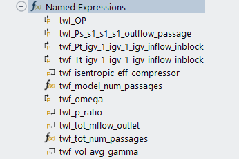
Double-click Named Expressions in the Outline View to open the Expression Manager where you can view the expression created by the Turbo Workflow. You can also edit the expression to make any modification for subsequent simulations. Select an expression from the Expressions list to see details of the expression definition.
For example, select twf_p_ratio to review its details.
Figure 12.7: The Expression Manager Dialog Box
You can also double-click an expression in the Outline View to display the Expression dialog box, where the expression is defined.
For example, double-click twf_p_ratio in the Outline View to display the Expression dialog box, where the pressure ratio named expression is defined as the ratio of the outlet pressure and the inlet pressure.
Figure 12.8: An Example of a Named Expression from the Turbo Workflow

12.4.4. Review Solution

12.4.4.1. Report Definitions

The workflow also automatically creates several report definitions, specific to the turbomachine analyses defined in the workflow.

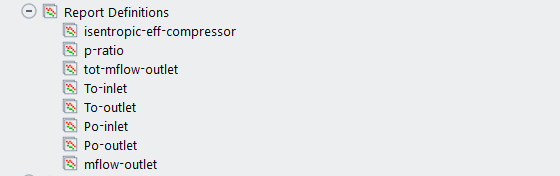
In the case of this axial compressor tutorial, the default report definitions created by the Turbo Workflow include:

isentropic-eff-compressor: the isentropic efficiency of the compressor
p-ratio: the ratio of the outlet pressure to the inlet pressure
tot-mflow-outlet: the total mass flow at the outlet
To-inlet: the total temperature at the inlet
To-outlet: the total temperature at the outlet
Po-inlet: the total pressure at the inlet
Po-outlet: the total pressure at the outlet
mflow-outlet: the mass flow at the outlet

Double-click Report Definitions in the Outline View to see a summary of each report definition in the Report Definitions dialog box.
Select p-ratio, for example, to see details of the its report definition, noting the creation and use of named expressions.
Figure 12.9: An Example of the Report Definitions Dialog Box
Double-click a report definition in the Outline View to see a summary of the definition.
For example, double-click p-ratio in the Outline View to display the Expression Report Definition dialog box where the pressure ratio between the outlet and the inlet is defined.
Figure 12.10: An Example of a Turbo-Specific Expression Report Definition

Note that report files and report plots have also been created for use in your turbomachinery simulation.
For more information about creating additional reports, see Solution of the Steady-State Mixing Plane Model in Modeling Blade Row Interaction using Steady-State and Transient Simulations.

12.4.4.2. Solution Controls

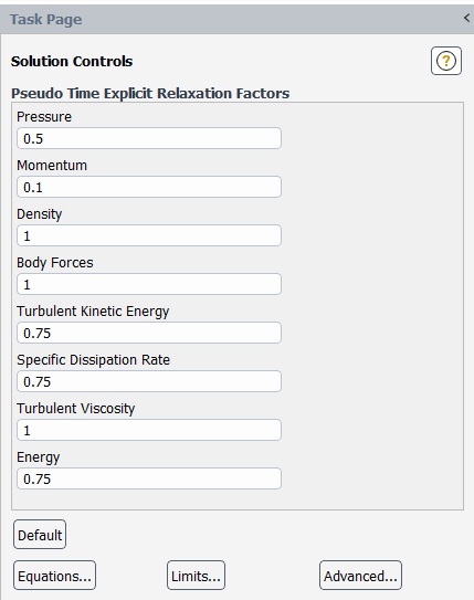
Change the Solution Controls for the Momentum equation (setting it to 0.1) to allow for a simulation run using a larger timescale.

Solution → Controls

12.4.4.3. Residual Monitors

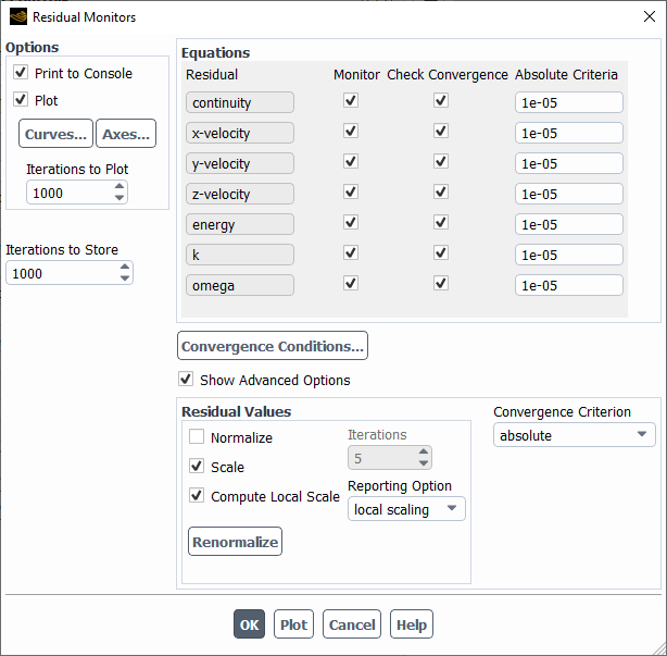
No changes are required for the Residual monitor settings, however, you should note how the settings have been changed from their default values and optimized for turbomachinery cases.

12.4.4.4. Monitors

The workflow also creates several report files and report plots, specific to the turbomachine analyses defined in the workflow.

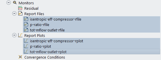
You will note the report files and plots correspond to the isentropic efficiency of the compressor, the pressure ratio, and the total mass flow rate at the outlet.

12.4.4.5. Solution

Perform a hybrid initialization of the flow field using the Initialization group box of the Solution ribbon tab.
Solution → Initialization
1. Select Hybrid from the Method list.
2. Click More Settings... to display the Hybrid Initialization dialog box.
  1. Set the Reference Frame to Absolute.
  2. Under Initialization Options, select Use Specified Initial Pressure on Inlets.
  3. Click Apply and close the Hybrid Initialization dialog box.
3. Note that the Initialize has already been performed as an automatic step in the Turbo Workflow.
Save the case and data file (turbo_workflow.cas.h5).
File → Write → Case and data ...
Start the calculation in the Solution ribbon tab (Run Calculation group box).
Solution → Run Calculation
1. Change the Time Scale Factor to 10.
2. Enter 200 for No. of Iterations.
3. Click Calculate to begin the iterations.
4. The residuals history will be plotted in the Scaled Residuals tab in the graphics window (Figure 12.11: Residuals).
  Figure 12.11: Residuals
5. The isentropic efficiency of the compressor will also be plotted in a separate tab in the graphics window (Figure 12.12: Isentropic Efficiency of the Compressor).
  Figure 12.12: Isentropic Efficiency of the Compressor
6. The pressure ratio will also be plotted in a separate tab in the graphics window (Figure 12.13: Pressure Ratio).
  Figure 12.13: Pressure Ratio
7. The total mass flow rate at the outlet will also be plotted in a separate tab in the graphics window (Figure 12.14: Total Mass Flow Rate at the Outlet).
  Figure 12.14: Total Mass Flow Rate at the Outlet
Save the case and data files (turbo_workflow.cas.h5 and turbo_workflow.dat.h5).
File → Write → Case & Data...

12.5. Postprocessing

Review the generated contour plots (velocity magnitude, Mach number, and the total pressure) along their span-wise locations.
Recall that the Turbo Workflow automatically creates contour plots at various span-wise locations, so you can easily review the flow field. These plots are available in the Results section once the solution is calculated.
Review the contours of the velocity magnitude at the initial span-wise location.
Results → Graphics → Contours → twf_velmag_twf_span_25

Click Save/Display and close the Contours dialog box.
Figure 12.15: Contours of Velocity Magnitude (span=25)

Perform the same operations for the other span-wise locations (twf_velmag_twf_span_50 and twf_velmag_twf_span_75).
Similarly, review the contours of total pressure at the initial span-wise location (twf_totpress_twf_span_25).
Figure 12.16: Contours of Total Pressure (span=25)

Perform the same operations for the other span-wise locations (twf_totpress_twf_span_50 and twf_totpress_twf_span_75).
Similarly, review the contours of Mach number at the initial span-wise location (twf_macnum_twf_span_25).
Figure 12.17: Contours of Mach Number (span=25)

Perform the same operations for the other span-wise locations (twf_macnum_twf_span_50 and twf_macnum_twf_span_75).

Compute and review the values for the named expressions.

In the Outline View, select all of the Named Expressions (selecting the first and then the last while holding the Shift key) . Right-click and select Compute from the context menu. The values for the named expressions will be tabulated in the console window.

------------------------------------------------------------------
                           Expression       Value Unit          
------------------------------------------------------------------
                               twf_OP           0 [kg m^-1 s^-2]
      twf_Ps_s1_s1_s1_outflow_passage       60500 [kg m^-1 s^-2]
twf_Pt_igv_1_igv_1_igv_inflow_inblock       60000 [kg m^-1 s^-2]
twf_Tt_igv_1_igv_1_igv_inflow_inblock      288.15 [K]           
        twf_isentropic_eff_compressor  0.85721193 []            
               twf_model_num_passages           1 []            
                            twf_omega    1790.708 [s^-1 rad]    
                          twf_p_ratio   1.2379454 []            
                 twf_tot_mflow_outlet  -7.9825762 [kg/s]        
                 twf_tot_num_passages          30 []            
                    twf_vol_avg_gamma   1.3990095 []            
------------------------------------------------------------------

Compute and review the values for the report definitions.

In the Outline View, select all of the Report Definitions (selecting the first and then the last while holding the Shift key). Right-click and select Compute from the context menu. The values for the report definitions will be tabulated in the console window.

        mflow-outlet
 -------------------
                  Mass Flow Rate              [kg/s]
-------------------------------- -------------------
           s1:s1-outflow-passage         -0.26608587

           Po-outlet
 -------------------
           Mass-Weighted Average                [Pa]
-------------------------------- -------------------
           s1:s1-outflow-passage           74276.727

            Po-inlet
 -------------------
           Mass-Weighted Average                [Pa]
-------------------------------- -------------------
        igv.1:igv-inflow-inblock               60000

           To-outlet
 -------------------
           Mass-Weighted Average                 [K]
-------------------------------- -------------------
           s1:s1-outflow-passage           309.24999

            To-inlet
 -------------------
           Mass-Weighted Average                 [K]
-------------------------------- -------------------
        igv.1:igv-inflow-inblock              288.15

    tot-mflow-outlet
 -------------------
                      Expression              [kg/s]
-------------------------------- -------------------
                tot-mflow-outlet          -7.9825762

             p-ratio
 -------------------
                      Expression                    
-------------------------------- -------------------
                         p-ratio           1.2379454

isentropic-eff-compressor
 -------------------
                      Expression                    
-------------------------------- -------------------
       isentropic-eff-compressor          0.85721193

Save the case and data files (turbo_workflow.cas.h5 and turbo_workflow.dat.h5).
File → Write → Case & Data...

12.6. Summary

In this tutorial, you learned how to use the Ansys Fluent Turbo Workflow to more easily set up a turbo-based fluid flow simulation to evaluate the performance of a compressor. Note that additional analysis of this same geometry can be found in Modeling Blade Row Interaction using Steady-State and Transient Simulations.