Modes to Terminals Conversion

This section describes the conversion of modal S-parameters, computed using HFSS's full-wave field solver, into terminal or voltage-based pseudo-S-parameters used in circuit theory.

The S-matrix solutions in HFSS are expressed in terms of incident and reflected complex amplitudes of waveguide modes. This description is mathematically and physically rigorous, but for the case of multi-conductor lines where multiples modes are propagating simultaneously it is convenient to convert the modes to physical quantities directly related to conductors such as currents. Examples of such situations include coupled transmission lines on printed circuit boards, multi-conductor cables, and many common types of electrical connectors. For these types of structures, which generally support multiple, quasi-transverse electromagnetic (TEM) modes of propagation, it is difficult to excite and measure a single mode. In any practical, or laboratory-like, measurement situation:

• measurements (e.g., voltage) contain contributions from several modes
• the applied stimuli excite several modes simultaneously

Terminal support was added to HFSS to enable the simulation of terminal currents and voltages directly, without requiring engineers to determine the needed linear combinations of waveguide modes.

Background

Recall from electromagnetic field theory that the solutions for the transverse components of the electric and magnetic fields in a waveguide with a uniform cross-section can be written as

		(1)
		(2)

Here the a_n and b_n are the intensities of the forward and backward traveling modal waves and are the transverse electric and magnetic field patterns. Note that the a_n and b_n are considered to be dimensionless quantities here, while and have the normal units for electric and magnetic fields. For this discussion's purpose, assume that each port is defined at z = 0; this permits the removal of exponential terms in the above equations.

Terminal Voltages and Currents

It is possible to define a set of voltages for a port by establishing a number of different integration paths across the port. If a port supports N quasi-TEM modes of propagation, one can set up N different open contours of integration, C₁, C₂, ... C_N, and define N different voltages, v₁, v₂, ... v_N, according to the integral formulas

Alternatively, you can define a set of currents {i_k}using a set of closed contours of integration {D_k}:

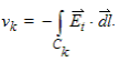		(3)
		(4)

These closed contour paths are set when you define the terminals on a port. HFSS does not require you to set up the voltage integration paths separately. The software automatically infers the voltage paths from the chosen current contours using a power conservation relationship.

Each definition produces a set of relationships between the modal intensities and the voltages or currents. Since the total transverse fields can be expanded as a linear combination of modes, we can rewrite the previous equations as

		(5)
		(6)

To simplify, introduce the following terms:

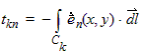		(7)
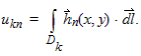		(8)

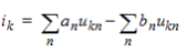
Now v_k and i_k become

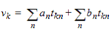		(9)
		(10)

Since there are N possible voltage definitions and N quasi-TEM modes, there are NxN matrices that relate the terminal voltages and currents to the following modal intensities:

		(11)
		(12)

Now introduce the matrices T = [t_kn] and U = [u_kn] to represent these transformations. Note that the units of T are volts, while the units of U are amperes.

In summary, the 3D Post Processor could be used to load different modal field patterns and manually perform the integrals defined previously over each terminal contour line. This would be a tedious and error-prone process, which HFSS's modes-to-terminals conversion feature eliminates.