VM-LSDYNA-DYNAMICS-003
VM-LSDYNA-DYNAMICS-003
Uniform Precession of Gyroscope (Elastic Shell Disk)
Overview
| Reference: | Kleppner, D., & Kolenkow, R. J. (2014). An introduction to mechanics (2nd ed.). McGraw-Hill Education, Singapore. (p. 300). |
| Analysis Type(s): | Explicit rotational dynamics |
| Analysis Component(s) |
A gyroscope (gyro) in uniform precession, elastic shell disk |
| Input Files: | Link to Input Files Download Page |
Test Case
The present finite element (FE) simulation calculates the precession angular speed Ω of a gyroscope (gyro) to validate the LS-DYNA dynamics calculations for spinning bodies, particularly rotational motion. All components, except for the elastic disk (flywheel), are modeled as rigid bodies. The precession is assumed to be uniform, although a slight nutation—cyclic nodding of the gyro—arises from imperfect initial conditions. In other words, the tip of the gyro axle is expected to swing at a constant rate. The numerical results are then compared with the analytical solution, showing strong agreement between the two approaches. In this study, the target quantity is the stabilized precession angular speed, Ω, of the horizontal gyro beam about the vertical z-axis Figure 388.
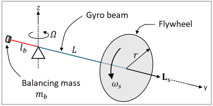
The simulation setup is schematically illustrated in Figure 388. The gyro flywheel is modeled as an elastic shell disk with a diameter of d = 2r = 0.1 m and a uniform shell thickness of t = 0.01 m, mounted to a rigid gyro beam at a distance of L = 0.205 m (in y direction) from the pivot. In this configuration, the flywheel spins rapidly about the gyro beam axis with a constant angular speed of ω = 1000 rad/s. The symbol LS denotes the gyroscope's spin angular momentum, generated entirely by this rotation, and directed along the flywheel axle as shown in Figure 388.
Figure 388: Schematic of the gyroscope (gyro) precession test case using elastic shell disk/flywheel
The table below shows the geometric properties, material properties, as well as loading and boundary conditions.
| Material Properties | Geometric Properties | Loading |
|---|---|---|
|
Density ρ = 7900 kg/m3 Young's modulus E = 2.1E+11 Pa Poisson's ratio ν = 0.30 |
Flywheel Diameter d = 0.1 m Thickness t = 0.01 m Gyro beam Gyro beam length l = 0.2 m Balancing Length lb = 0.05 m |
Gravity g = 9.81 m/s2 Initial angular rotation of gyro Ω0 = 1.4 rad/s Flywheel angular speed ωs = 1000 rad/s Balancing mass mb ≈ 0.3 kg |
Analysis Assumptions
It is known that  , where
  is the moment of inertia of the flywheel about the gyro axle and
 is the constant flywheel angular speed. Given this, the angular velocity of
precession
is the constant flywheel angular speed. Given this, the angular velocity of
precession  is calculated as
 | (149) |
where  is the flywheel weight and
  denotes the distance between the shell disk and the pivot. Since
 , where
  is the disk mass, for the present disk,
 | (150) |
Substituting Equation 150 into Equation 149 gives
 | (151) |
As Equation 151 shows, the disk mass
 is cancelled out from the numerator and the denominator. For the present
case, implementing
is cancelled out from the numerator and the denominator. For the present
case, implementing  = 0.205 m, g ≈ 9.81 (m/s2),
  = 1000 rad/s, and
  = 0.05 m yields an analytical value of = 1.61 rad/s.
Equation 151 is derived under the assumption that the gyro axis (the rigid beam) does not contribute to any torque—that is, it is considered massless. However, in the present model the beams are not massless. To eliminate this torque, as schematically illustrated in Figure 388, a counterweight of mass mb is added to the opposite end, with a balancing beam length of lb = 0.05 m (shown red), so that the beam remains roughly balanced when the gyro is removed. This balance can be verified in the d3hsp file by inspecting Part 4 (the gyro beam) and checking the center of mass, which is found to be very close to (0,0,0), the mounting point of the beam, in the present case using mb ≈ 0.3 kg and lb = 0.05 m.
Modeling Notes
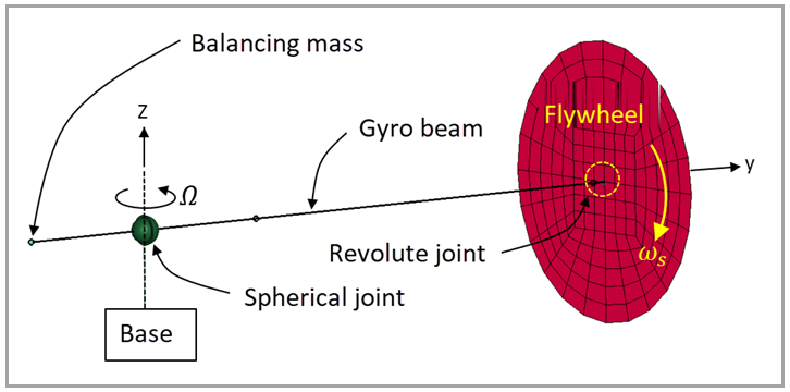
The deformable flywheel is modeled in LS-DYNA using the *MAT_001/*MAT_ELASTIC material model, with a density of 7900 kg/m³, a Young’s modulus of 2.1E+11 Pa, and a Poisson's ratio of 0.3. As shown in Figure 389, the flywheel (gyro disk) is discretized using quadrilateral shell elements, while the gyro axle is represented by beam elements. Element formulations ELFORM = 16 (fully integrated shell element modified for higher accuracy) and ELFORM = 1 (Hughes-Liu with cross section integration) are applied to the flywheel and axle, respectively. The constant angular speed of the flywheel about the axle (ωs = 1000 rad/s) is imposed using OMEGA in *INITIAL_VELOCITY_GENERATION. This spin rate is chosen to be much greater than the analytical precession angular speed, Ω = 1.61 rad/s, of the gyro beam about the z-axis, ensuring the expected gyroscopic precession behavior.
The axle is connected to the flywheel via *CONSTRAINED_JOINT_REVOLUTE and to the base via *CONSTRAINED_JOINT_SPHERICAL. The revolute joint between the beam and the shell disk is defined using two coincident node pairs that establish the hinge axis. The first pair is taken directly from the natural intersection of the beam and the disk, where the beam node and the shell node already coincide in space. The second pair is formed by selecting another node along the beam axis (for example, the beam end node) and creating a single dummy node on the disk side at the exact same coordinates. Since this dummy node has no element connectivity, it is tied to the deformable disk through a local nodal rigid body (*CONSTRAINED_NODAL_RIGID_BODY) that includes the dummy node together with a small set of nearby shell nodes from the disk, ensuring that the dummy node follows the disk’s motion while the rest of the disk remains deformable. These two coincident pairs are then specified in the *CONSTRAINED_JOINT_REVOLUTE keyword, which constrains all relative motion between the beam and the disk except for rotation about the axis defined by the two pairs, thereby implementing the desired hinge behavior.
To reduce the amplitude of the nutation effect, the gyro is also given an initial angular
velocity of  = 1.4 rad/s around the z-axis via
*BOUNDARY_PRESCRIBED_MOTION_RIGID_LOCAL, applied with a short
deactivation time of 0.02 s. The nutation effect is a real physical
phenomenon, not a numerical artifact. This effect is characterized by the repeated nodding
motion of beam Part 4. Adjusting the initial value
Ω0 can be used to reduce this effect. In this simulation, the
total run time is set to 2 s, and the SI unit system (kg, m, s, N, Pa) is
used, although the model can be adapted to any consistent unit system if required.
= 1.4 rad/s around the z-axis via
*BOUNDARY_PRESCRIBED_MOTION_RIGID_LOCAL, applied with a short
deactivation time of 0.02 s. The nutation effect is a real physical
phenomenon, not a numerical artifact. This effect is characterized by the repeated nodding
motion of beam Part 4. Adjusting the initial value
Ω0 can be used to reduce this effect. In this simulation, the
total run time is set to 2 s, and the SI unit system (kg, m, s, N, Pa) is
used, although the model can be adapted to any consistent unit system if required.
Figure 389: Model setup for the gyroscope precession simulation in LS-DYNA using elastic shell disk/flywheel
Results Comparison
To verify the accuracy of the simulation and the reliability of the LS-DYNA’s dynamic calculations, the predicted value of the target parameter is compared against the analytical solution. Here, the target parameter is the stabilized precession angular speed Ω (rad/s). This is obtained by averaging the angular velocity of the horizontal gyro beam about the z-axis. Specifically, the z-angular velocity of Part 4 (component: global_rvz in rbdout) is extracted from the binout file and plotted, as shown in Figure 390. If necessary, the sinusoidal signal can be smoothed using a Butterworth filter (bw) with a cutoff frequency of 60 Hz to reduce small system oscillations. The average z-angular velocity is then computed after 1.5 s (shaded-yellow in Figure 390), once the motion has stabilized. As summarized in the results table below, the simulation predicts 1.59 ± 0.21 rad/s, corresponding to a deviation of -1.24% from the analytical value. It is noted that a coarser mesh would increase the discrepancy between the analytical and numerical moments of inertia, thereby reducing the agreement between the two methods. The double-precision version of LS-DYNA is required to run this model. Using the single-precision version may eventually cause the simulation to degenerate (for example, after approximately 400,000 cycles).
The following table shows the predicted value of the stabilized precession angular speed versus the analytical solution.
| Result | Target | LS-DYNA | Error (%) |
|---|---|---|---|
|
Stabilized angular speed of precession Ω (rad/s) | 1.61 | 1.59 | -1.24 |
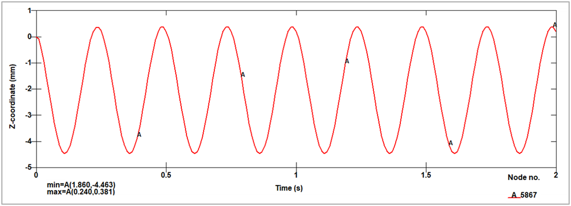
Figure 390 plots the history of the z-angular velocity of elastic shell disk (global_rvz of Part 4 in rbdout) from the binout file, showing the stabilized precession rate and nutation oscillations. In this case Ω0 = 1.4 rad/s. The sinusoidal behavior of the curve represents the nutation effect observed in the present simulation. This is a real physical phenomenon (rather than a numerical artifact) characterized by a slight oscillatory nodding of the gyroscope's axis superimposed on the uniform precession motion. To reduce this effect in the current case, and make it close to the ideal uniform precession, the initial precession angular velocity Ω0 is set to 1.4 rad/s, a value close to the analytical prediction of 1.61 rad/s for the stabilized precession angular velocity Ω. In the spatial domain, nutation appears as a periodic variation in the flywheel's vertical (z) coordinate between approximately −4.5 mm and 0.4 mm (Figure 391). You can adjust the initial conditions, particularly the imposed initial precession angular velocity Ω0 to further reduce the oscillation amplitude of the nutation effect.
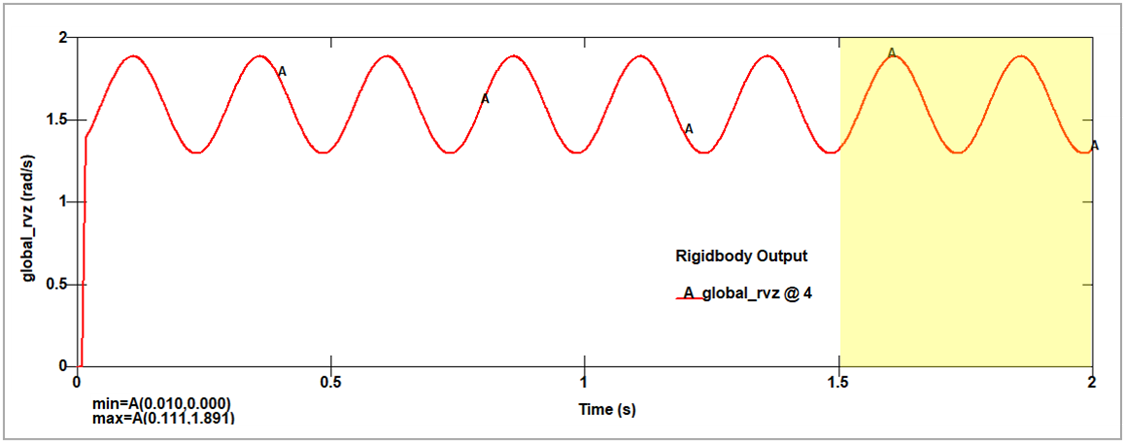
Figure 391 plots the history of the flywheel's vertical (z) coordinate, illustrating periodic nutation motion with amplitude ranging from approximately −4.5 mm to 0.4 mm. In this case, Ω0 = 1.4 rad/s.