VM-LSDYNA-DYNAMICS-001
VM-LSDYNA-DYNAMICS-001
Uniform Precession of Gyroscope (Rigid Parts)
Overview
| Reference: | Kleppner, D. & Kolenkow, R. J. (2014). An introduction to mechanics (2nd ed.). McGraw-Hill Education, Singapore. (p.300). |
| Analysis Type(s): | Explicit rotational dynamics |
| Analysis Component(s): | A gyroscope (gyro) in uniform precession, rigid parts |
| Input Files: | Link to Input Files Download Page |
Test Case
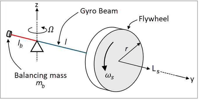
The present finite element (FE) simulation calculates the precession angular speed Ω of a gyroscope (gyro) to validate LS-DYNA's dynamics calculations for spinning bodies, specifically rotational motion. All components are modeled as rigid bodies, and the precession is assumed uniform although there is a slight nutation of the gyro (cyclic nodding) due to the imperfect initial conditions—that is to say, the tip of the gyro axle is expected to swing at a constant rate. The numerical results are then compared with the analytical solution, demonstrating the strong agreement between the two approaches. In this study, the target quantity is the stabilized precession angular speed Ω of the horizontal gyro beam about the vertical z-axis. See Figure 379.
The simulation setup is schematically illustrated in Figure 379. The gyro flywheel is modeled as a rigid disk with a diameter of d = 2r = 0.1 m and a uniform thickness of t = 0.01 m, mounted to a rigid gyro beam at a distance of l = 0.2 m from the pivot—that is, l is the distance between the most left face of the disk (in the y direction) and the pivot. In this configuration, the flywheel spins rapidly about the gyro beam axis with a constant angular speed of ωs = 1000 rad/s. The symbol Ls denotes the gyroscope's spin angular momentum, generated entirely by this rotation, and directed along the flywheel axle as shown in Figure 379.
The table below shows the geometric properties, material properties, as well as loading and boundary conditions.
| Material Properties | Geometric Properties | Loading |
|---|---|---|
|
Density ρ = 7900 kg/m3 Young's modulus E = 2.1E+11 Pa Poisson's ratio ν = 0.30 |
Flywheel Diameter d = 0.1 m Thickness t = 0.01 m Gyro beam Gyro beam length l = 0.2 m Balancing length lb = 0.05 m |
Gravity g = 9.81 m/s2 Initial angular rotation of gyro Ω0 = 1.4 rad/s Flywheel angular speed ωs = 1000 rad/s Balancing mass mb ≈ 0.3 kg |
Analysis Assumptions
It is known that  , where
  is the moment of inertia of the flywheel about the gyro axle and
 is the constant flywheel angular speed. Given this, the angular velocity of
precession
is the constant flywheel angular speed. Given this, the angular velocity of
precession  is calculated as
 | (143) |
where  is the flywheel weight and
  . Here,
  denotes the distance between the CG (center of gravity) of the disk and the
pivot. Since
denotes the distance between the CG (center of gravity) of the disk and the
pivot. Since  , where
  is the disk mass for the present disk,
 | (144) |
Substituting Equation 144 into Equation 143 gives
 | (145) |
As Equation 145 shows, the disk mass
 is cancelled out from the numerator and the denominator. For the present
case, implementing =
0.205 m,
is cancelled out from the numerator and the denominator. For the present
case, implementing =
0.205 m,  ≈ 9.81 (m/s2),
  = 1000 rad/s, and
  = 0.05 m yields an analytical value of =
1.61 rad/s.
= 0.05 m yields an analytical value of =
1.61 rad/s.
Equation 145 is derived under the assumption that the gyro axis (the rigid beam) does not contribute to any torque—that is, it is considered massless. However, in the present model the beams are not massless. To eliminate this torque, as schematically illustrated in Figure 379, a counterweight of mass mb is added to the opposite end, with a balancing beam length of lb= 0.05 m (shown red), so that the beam remains roughly balanced when the gyro is removed. This balance can be verified in the d3hsp file by inspecting Part 4 (the gyro beam) and checking the center of mass, which is found to be very close to (0,0,0), the mounting point of the beam, in the present case using mb ≈ 0.3 kg and lb = 0.05 m.
Modeling Notes
The non-deformable flywheel is modeled in LS-DYNA using the
*MAT_020/*MAT_RIGID material model, with a density of
7900 kg/m³, a Young's modulus of 2.1E+11 Pa, and a
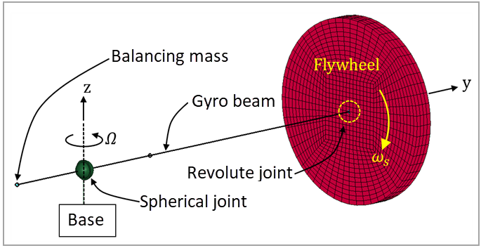
Poisson's ratio of 0.3. As shown in Figure 380, the flywheel (gyro plate) is discretized using fine hexahedral
solid elements, while the gyro axle is represented by beam elements. Element formulations
ELFORM = 2 (8-point hexahedron) and ELFORM = 1
(Hughes-Liu with cross section integration) are applied to the flywheel and axle,
respectively. The axle is connected to the flywheel via
*CONSTRAINED_JOINT_REVOLUTE and to the base via
*CONSTRAINED_JOINT_SPHERICAL. The constant angular speed of the
flywheel about the axle ( = 1000 rad/s) is imposed using OMEGA in
*INITIAL_VELOCITY_GENERATION. This spin rate is chosen to be much
greater than the analytical precession angular speed, =
1.61 rad/s, of the gyro beam about the z-axis, ensuring the expected
gyroscopic precession behavior.
To reduce the amplitude of the nutation effect, the gyro is also given an initial angular velocity of Ω0 = 1.4 rad/s around the z-axis via *BOUNDARY_PRESCRIBED_MOTION_RIGID_LOCAL, applied with a short deactivation time of 0.02 s. The nutation effect is a real physical phenomenon, not a numerical artifact. This effect is characterized by the repeated nodding motion of beam Part 4. Adjusting the initial value Ω0 can be used to reduce this effect. In this simulation, the total run time is set to 2 s, and the SI unit system (kg, m, s, N, Pa) is used, although the model can be adapted to any consistent unit system if required.
Figure 380: Model setup for the gyroscope precession simulation in LS-DYNA using rigid flywheel/disk
Results Comparison
To verify the accuracy of the simulation and the reliability of the LS-DYNA's dynamic calculations, the predicted value of the target parameter is compared against the analytical solution. Here, the target parameter is the stabilized precession angular speed, Ω (rad/s). This is obtained by averaging the angular velocity of the horizontal gyro beam about the z-axis. Specifically, the z-angular velocity of Part 4 (component global_rvz in rbdout) is extracted from the binout file and plotted, as shown in Figure 381. If necessary, the sinusoidal signal can be smoothed using a Butterworth filter (bw) with a cutoff frequency of 60 Hz to reduce small system oscillations. The average z-angular velocity is then computed after 1.5 s (shaded yellow) in Figure 381), once the motion has stabilized. As summarized in the results table below, the simulation predicts 1.61 ± 0.22 rad/s, corresponding to no deviation from the analytical value. An exact match (zero discrepancy) was achieved by using a sufficiently fine mesh. In contrast, a coarser mesh would increase the discrepancy between the analytical and numerical moments of inertia, thereby reducing the agreement between the two methods.
| Results | Target | LS-DYNA Solver | Error (%) |
|---|---|---|---|
|
Stabilized angular speed of precession Ω (rad/s) | 1.61 | 1.61 | 0.00 |
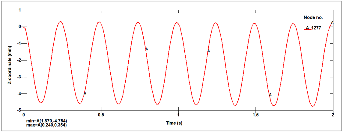
Figure 381 shows the history of the z-angular velocity of rigid disk (global_rvz of Part in rbdout) from the binout file, showing the stabilized precession rate and nutation oscillations. In this case, Ω0 = 1.4 rad/s. The sinusoidal behavior of the curve represents the nutation effect. This is a real physical phenomenon (rather than a numerical artifact) characterized by a slight oscillatory nodding of the gyroscope's axis superimposed on the uniform precession motion. To reduce this effect in the current case, and make it close to the ideal uniform precession, the initial precession angular velocity, Ω0, is set to 1.4 rad/s, a value close to the analytical prediction of 1.61 rad/s for the stabilized precession angular velocity Ω. Increasing Ω0 from 1.0 rad/s to 1.4 rad/s did not change the predicted mean value of Ω (1.61 rad/s), but it reduced the standard deviation from 0.47 rad/s to 0.22 rad/s, which provides a quantitative measure of the nutation intensity. In the spatial domain, nutation appears as a periodic variation in the flywheel's vertical (z) coordinate between approximately −4.8 mm and 0.4 mm (Figure 382). Typical nutation moments (that is, when the flywheel's z-position exceeds the initial reference lines) are shown in Figure 383. You can adjust the initial conditions, particularly the imposed initial precession angular velocity Ω0 to further reduce the oscillation amplitude.
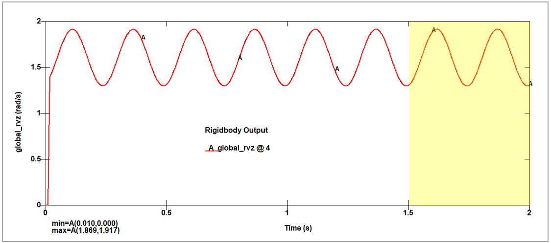
Figure 382 shows the time history of the flywheel's vertical (z) coordinate, illustrating periodic nutation motion with amplitude ranging from approximately −4.8 mm to 0.4 mm. In this case, Ω0 = 1.4 rad/s.
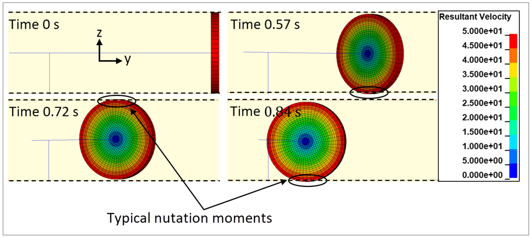
Figure 383 shows snapshots of typical nutation moments during the simulation, showing instances where the flywheel's vertical (z) position exceeds the reference z lines (dashed) while the gyroscope rotates counterclockwise (CCW) in the x-y plane. In this case, Ω0 = 1.4 rad/s.