Fluent Guided Meshing Workflows

• The Watertight Geometry Workflow

  • Stairstep options for thin volume meshing have been deprecated.

  • The parallel region compute option for conformal regions has been added to the Generate the Surface Mesh task, resulting in improved performance for cases with many objects.

  • The following additional controls are now available in the Extrude Volume Mesh task for extruding periodic zones:

    • Extend to Periodic Pair

    • Extend Periodic

    • Max Layer Height

  • In the Add Local Sizing task, the Ignore Proximity Across Objects option has been added for controlling proximity size using faces only.

  • Autodetection of thin regions has been improved for thin volume meshing. Auto-separated source and target zones created during thin volume detection are now automatically merged at the end of volume meshing, resulting in fewer zones and boundary condition settings in the solver compared to previous releases.

• The Fault-tolerant Meshing Workflow

  • The CAD Assemblies capability has been deprecated and will be removed in a future release. For similar capability consider using the Part Management capabilities.

  • In the Add Boundary Layers task, label(s) that have already been assigned boundary layers will no longer be available in the list of named label(s).

  • placeholder

• The 2D Meshing Workflow

  • The Axisymmetric Sweep task has been added to the workflow and can be used to create a 3D mesh by revolving a 2D axisymmetric mesh about a specified axis.

Mesh Generation

• When using curvature size functions with the Rapid Octree mesher, the following are now supported as full features:

  • You now have the ability to change the criterion used for the refinement of the curved surfaces. The new choices—switched (which is now the default) or arc-estimate—are less sensitive to surface faceting and can provide refinement even as the facet resolution increases compared to facets-normal-angle (the default in previous releases). If you want to revert to the criterion used in previous releases in order to maintain the same cell counts, you can use the following text command: mesh/rapid-octree/mesh-sizing/curvature-refinement-options/criterion facets-normal-angle

  • You can now set maximum and minimum angle thresholds between the two facets for angular refinements with curvature size functions; such settings can be useful, for example, to exclude sharp corners and to prevent spurious refinements, respectively.

  For further details, see Creating Size Functions.

User Experience

• Search is now available for filtering contents in both Preferences and the Console.

• The Raytracing Display window, where realistic images and volume renders are displayed, now accepts graphics manipulations such as pan, rotate, and zoom. Refer to Realistic Rendering Using Raytracing in the Fluent User's Guide to learn more about these types of displays.

Third-party Software

• HOOPS is now updated to 30.14 from 27.23 to address security vulnerabilities.

Solver-Meshing

• When using overset meshes, the Green-Gauss Node Based gradient scheme is now supported with both the pressure-based solver and the density-based solver. (Overset Meshing Limitations and Compatibilities)

• When using a mesh interface with the Green-Gauss Node Based gradient scheme, a new expert option is available that allows you to control the enforcing of bounds on interpolation weights for solution variables at the nodes of non-conformal interface boundaries. You can enter the following text command to disable the clipping of the node interpolation weights, which can improve the quality of gradients at the cells adjacent to the non-conformal interfaces: solve/set/gradient-options/green-gauss-node-based/weight-treatment-at-sliding-boundary? yes.

• The following improvements are available when you create a non-conformal mesh interface using the default one-to-one interface creation method:

  • A list is now automatically printed in the console for any associated boundary zone that is deemed to be over-intersected (that is, a boundary zone that has at least one face in which the total intersection area for the face is bigger than the area of that face multiplied by a factor of 1.25), along with metrics that indicate the extent of the over-intersection. This information is also printed if you list the details of an existing mesh interface. You should investigate all over-intersected boundary zones, to confirm if their mesh interfaces are properly defined.

  • You can now specify whether the lists of mesh interfaces printed in the console are ordered by their overlap area (that is, the area that the two boundary zones overlap) or by their overlap area percentage (that is, the overlap area divided by the area of each of the two boundary zones). Previously the lists were always ordered by the overlap area percentage.

  • You can now define a minimum area of overlap that is used to create mesh interfaces when zones are paired using the automatic method. This can help you avoid unnecessary or unintentional mesh interfaces. Previously you could only define a minimum overlap area percentage.

  • When you are deleting existing mesh interfaces that have small overlap, you can now specify an area that is used for deletion: if the area that the two boundary zones overlap for any mesh interface is less than this value, then it will be deleted. Previously you could only specify an overlap area percentage for deletion.

  • The non-conformal interface surfaces from one-to-one mesh interfaces now participate in postprocessing operations. Note that for the non-overlapping face zones, the faces adjacent to the intersected zone will only be displayed or contribute to integrals if they are sufficiently large compared to their parent faces (and then the parent faces will be used).

  For details about non-conformal mesh interfaces, see Using a Non-Conformal Mesh in Ansys Fluent.

• The following improvements are now available when deleting or deactivating cell zones:

  • You can now delete or deactivate a cell zone with boundary zones that are non-manifold. This was previously possible in the meshing mode of Fluent and is now also supported in the solution mode. This can be useful when postprocessing for example, as you can visualize a single small zone by deactivating all of the other zones.

  • Fluent now robustly handles attempts to delete or deactivate a cell zone with a boundary zone that has misoriented faces; while such an action has never been and is still not fully supported, it will no longer result in a broken mesh or the abnormal termination of Fluent, and this allows you proceed using Scheme commands at your own risk (as noted in warning messages in the console).

  For details about deleting and deactivating cell zones, see Deleting Zones and Deactivating Zones, respectively.

• It is now possible to extract cells that are marked by a specified cell register (as well as any specified additional layers of neighboring cells), so that they are preserved and all other cells in the mesh are deleted. Extracting cells can be useful when working with a large mesh that is difficult to manipulate, as it can allow you to focus on a small region of interest and easily perform actions such as postprocessing. (Extracting Cells)

• You can now easily fuse all of the contacting face zones between selected cell zones, rather than having to select all of the individual face zones. This is particularly useful if you have disconnected cell zones and want to reestablish connection. (Fusing Face Zones of Selected Cell Zones)

• The ability to project the nodes from one or more boundary zones so that they are moved to be coincident with an auxiliary geometry definition is now supported as a full feature. This can be useful for sliding mesh simulations, as you can make sure that all of the nodes of a boundary pair for the non-conformal interface are on the same plane or on the same surface, in order to reduce simulation errors. (Projecting Boundary Zones Onto an Auxiliary Geometry Definition)

Cell Zones and Boundary Conditions

• When using the pressure-based solver with a turbulence model, a treatment option is now enabled by default, such that the effects of turbulence wall functions are removed at walls where you have specified zero shear. This treatment applies the Neumann boundary condition for the turbulence quantities, so that the walls behave as symmetric boundary conditions. This enhances the convergence, as no turbulence wall modeling is performed. It is possible that this treatment may make minor changes to the solution near the wall, but they should not be meaningful. You can disable this treatment by entering the following text command: solve/set/advanced/specified-zero-shear-alternative-treatment? no. (Specified Shear)

• When using the pressure-based solver, a new treatment is applied by default to the following boundary conditions, in order to avoid inaccurate flow prediction when the direction specified is not well aligned with the local boundary face normal:

  • pressure inlets with Direction Vector selected from the Direction Specification Method drop-down list (see Pressure Inlet Boundary Conditions)

  • pressure outlets that: have the Prevent Reverse Flow option disabled; have either Direction Vector or From Neighboring Cell selected from the Backflow Direction Specification Method drop-down list; and experience backflow conditions (see Pressure Outlet Boundary Conditions)

  If you do not want to take advantage of this increased accuracy, you can undo the default treatment for pressure inlets and pressure outlets with misaligned directions using the appropriate prompt of the following text command: solve/set/previous-defaults/undo-2026r1-default-changes?.

Heat Transfer / Radiation

• You can now model ambient radiation to the external environment without needing to create a fluid box around the geometry. This significantly simplifies the case set up by eliminating the need to mesh/model the fluid medium between surfaces and can also significantly reduce computation time. (Ambient Radiation Modelling)

• The Macro heat exchanger model now supports non-conformal interfaces at flow inlets and outlets.

Turbulence

• The original version of the GEKO model (GEKO_2015) has shown some conceptual weaknesses which have motivated a moderate re-formulation (GEKO_2024) in order to improve tuning capabilities. The main issue was the need to separate the tuning coefficients of the model between coefficients affecting boundary layers and coefficients affecting frees shear flows.

  The improved GEKO_2024 is the default GEKO model version in 2026 R1. The original GEKO_2015 is still available, but the recommended model version is GEKO_2024.

  Note that in .cas files created with Fluent versions previous to 2026 R1 which not have GEKO enabled, the default GEKO version will be set to 2024 in the background and version dependent coefficients (CMIX, CJET and CJET_AUX) will be adjusted to their default values.(Generalized k-ω  (GEKO) Model)

• For the WALE LES model, the turbulence length scale is now limited close to the walls for high aspect ratio meshes. This improves solver stability for cases with poor mesh quality and without influencing the solution and separation prediction on isotropic meshes. (Wall-Adapting Local Eddy-Viscosity (WALE) Model)

• When using the GPU solver with the LES model, for near-wall treatment, you can now have the input fields used for wall-function evaluation be taken from the second cell off the wall. (Features Supported by the Fluent GPU Solver)

• When using the GPU solver with either the kω-SST or GEKO models, the tabulated Near-Wall Treatment is now available in addition to the correlation method. (y+-Insensitive Near-Wall Treatment for ω-based Turbulence Models)

Turbo Setup Workflow

• Performance gains have been notably improved when copying and merging multiple cell zones in the Turbo Setup Workflow.

Discrete Phase Model

• For simulations that involve the Lagrangian wall film (LWF), a new caloric temperature treatment is now available for the film temperature calculation. The treatment provides improved accuracy in cases where:

  • the particle material has temperature-dependent specific heat

  • the film consists of two or more materials with different physical properties that coexist on the same wall face

  For more information, see Calculation of Wall Film Face Variables in the Fluent Theory Guide.

• In coupled simulations with the GPU solver, the Linearize Source Terms option is now fully supported for species sources.

• In simulations with the GPU solver where particle species are evaporating, the binary diffusivity of the particle material can now be modeled using the film-averaged approach.

• For cases involving the film-to-wall heat transfer model, you can now specify the distance between the film starting position and the heat transfer region. This capability can significantly improve the accuracy of convective film heat transfer simulations, particularly when the film start point is upstream of the heat transfer region. (Setting the Film-to-Wall Heat Transfer Model)

Multiphase Models

• A text command, solve/set/multiphase-numerics/interphase-interactions/turbulent-dispersion/disable-turbulent-dispersion-next-to-flow-boundaries?, is now available for disabling momentum sources due to turbulence-dispersion in cells next to flow boundaries. In certain cases this can significantly improve convergence.

• For Eulerian multiphase cases that involve the critical heat flux (CHF) boiling model, droplet diameters for the primary phase can now be modeled as a constant or using the bending diameter model. (Procedure for Setting the Boiling Model in the Fluent User's Guide)

• For the wall boiling model, a new text command, solve/set/multiphase-numerics/boiling-parameters/bubble-diameter-model-options, has been added. The command allows you to select between the default and Unal bubble diameter modeling options. This functionality was accessed through a scheme command in previous releases.

• For multiphase species-transport simulations, a vanishing phase treatment has been introduced. The treatment respects initial mass fraction values in cases where phase change depends on partial pressure or where species transfer occurs between phases. (Modeling Multiphase Species Transport)

Electric Potential Field and Electrochemistry Model

• The Electrolysis and H2 Pump Model has been renamed Electrochemical Devices and has been enhanced with the following capabilities:

  • The following new device types have been introduced:

    • Solid oxide fuel cell (SOFC)

    • Solid oxide electrolysis cell (SOEC)

    • Customized electrochemical reactions

    See Electrochemical Devices in the Fluent Theory Guide for details.

  • The ability to account for species diffusion through the membrane of electrochemical devices has been added. (Setting Advanced Options (Advanced Tab))

  • In the unresolved electrochemistry model, you can now customize the membrane electrolyte conductivity via the DEFINE_ELECTROLYSIS_COND user-defined function (UDF). For details, see DEFINE_ELECTROLYSIS_COND in the Fluent Customization Manual.

• For the Lithium-ion battery model, the following additional postprocessing quantities are now available in the Lithium... category:

  • Overpotential in Li-Intercalation Reaction

  • Overpotential in SEI Growth Reaction (aging model)

  • Overpotential in Li-Plating Reaction (aging model)

  For definitions of these field variables, refer to Alphabetical Listing of Field Variables and Their Definitions in the Fluent User's Guide.

Battery Model

• The following battery modeling capabilities are now supported with the GPU solver:

  • CHT Coupling solution method

  • Joule Heat in Passive Zones energy source option

  • Battery ROM tool kit

• For the Newman's P2D model, you can now import model parameters from a BPX-format JSON file using the BPX file reader. (Inputs for the Newman’s P2D Model)

• When using the ROM tool kit, you can now specify a heat flux distribution on selected walls (Create ROM Training Data (ROM Data Creator Tab))

• For the one-equation thermal abuse model, the parameter estimation tool is now available in the graphical user interface (GUI). Consequently, the Standalone Thermal Abuse Model dialog box has been renamed to Fitting Tool/Standalone Thermal Abuse Model, and the Preview Thermal Abuse Model... button in the Battery Model dialog box (Advanced tab) has been renamed to Fitting Tool/Standalone Model.... (Fitting Tool/Standalone Thermal Abuse Model)

Proton Exchange Membrane Fuel Cell (PEMFC) Module

• The degradation model to simulate degradation processes in the membrane is now available. (Setting Material Chemical Degradation)

Solver

• When using the Green-Gauss Node Based gradient scheme, the improved treatment of symmetry and periodic boundaries in the node-based reconstruction gradient is now available for the pressure-based solver. This treatment ensures that the gradient respects symmetry and periodic constraints at the discrete level, thus better matching results obtained on an untruncated domain. (Green-Gauss Node-Based Gradient Evaluation)

• When using the pressure-based solver, you can now use a user-specified gradient scheme to compute the reconstruction gradient that is used in the second-order pressure interpolation. This allows better accuracy of the second-order scheme compared to the current default (which is based on the Green-Gauss Cell Based scheme for general unstructured meshes). To use the user-specified gradient scheme, enter the following text command: solve/set/gradient-options/pressure-reconstruction-type? yes.

• When using the Least Squares Cell Based gradient, you can now control the weighting factor used in the assembly of the least squares matrix system that computes the gradient weights. You can specify that the weighting factor is unweighted, inverse distance weighted, or the default inverse distance squared weighted. The use of unweighted or inverse distance weighted may result in improved accuracy, especially at physical boundaries. To specify the weighting factor, use the following text command: solve/set/gradient-options/least-squares/weighting-factor.

• When using the pressure-based solver, you can now apply the PRESTO! pressure interpolation treatment at fluid physical boundaries. This is intended to be used with any other pressure interpolation scheme besides PRESTO!, in order to improve the flow prediction without being subject to the mesh size sensitivity of the PRESTO! scheme. (Choosing the Pressure Interpolation Scheme)

• You can now specify the use of the bi-conjugate gradient stabilized method (BCGSTAB) for the energy equation in all future sessions of Fluent by enabling the BCGSTAB for Energy Equation option in the Simulation branch of the Preferences dialog box (accessed through File/Preferences...). This can be helpful with conjugate heat transfer (CHT) problems, as described in Conjugate Heat Transfer. For further details about the BCGSTAB method, see Setting the Stabilization Method.

Fluent Native GPU Solver

• The following improvements are available when using expressions for report definitions and unsteady statistics with the GPU solver:

  • Additional fields are now supported as a full feature for fully supported models, including fields for material properties, turbulence modeling, reaction and combustion, the volume of fluid (VOF) model, and user-defined scalars (UDS). For the full list of supported fields and other details, see Using Expressions with Report Definitions and Unsteady Statistics.

  • When creating an expression report definition, the selection of existing report definitions as part of the definition is now supported. For further details, see Using Expressions with Report Definitions and Unsteady Statistics.

• When using the GPU solver, CPU/GPU remapping is now supported with asynchronous (async) outputting, as long as the case does not have a command defined through the Execute Commands dialog box for execution during the calculation that requires downloaded data from the GPU. For further details about these features, see CPU/GPU Remapping and Asynchronous Outputting, respectively.

• When using the GPU solver, asynchronous (async) outputting is now supported when automatically exporting solution data as EnSight DVS files during a calculation. For further details about these features, see Asynchronous Outputting and Exporting Solution Data as EnSight DVS Files, respectively.

• The GPU Solver can now be started in hybrid precision, resulting in improved performance and memory consumption when compared to the double precision solver.

• Supersonic inflow (ideal gas only) is now supported at velocity inlets and mass flow inlets.

• For the Potential/Electrochemistry model, time-dependent values and contact resistance can now be specified at wall boundaries.

• Vertex Average, Vertex Minimum, and Vertex Maximum monitors can now be defined on zone, point, and plane surfaces.

• Monitors can now be defined on iso-surfaces.

Graphics, Reporting, and Postprocessing

• You can create key frame-based animations without having a case or data file loaded by using HSF animation files. Refer to HSF File and In Memory Key Frames in the Fluent User's Guide for additional information.

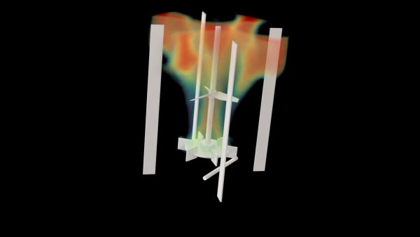
• Volume rendering is now full feature, allowing you to create images like Figure 2.1: Example Volume Rendering with Mesh. These volumes can also be included within animation definitions. Refer to Displaying Volume Renderings in the Fluent User's Guide for additional information.

  Figure 2.1: Example Volume Rendering with Mesh

  
  
  

• You can now create new and access existing graphics objects (such as contours, vectors, pathlines, and so on) prior to reading a data file or initializing the flow field.

• The import of STL surfaces is now done through the External Surface dialog box. This new approach (previously import was done using the Imprint Surface dialog box) uses a better algorithm that results in superior data mapping. Refer to External Surfaces in the Fluent User's Guide for additional information.

• You can now split surfaces, such as planes or external surfaces, at each location where that surface crosses a boundary, allowing for greater granularity in postprocessing. Refer to Split Surfaces in the Fluent User's Guide for additional information.

• The iso-surface and iso-clip algorithm is improved.

  • For iso-surfaces, it offers improved performance, particularly when creating multiple surfaces at once. It also has improved handling of boundaries during surface creation.

  • For iso-clips, faceting is improved.

Adjoint Solver Module

• The prescribed profile boundary condition within the design tool can now be defined using an expression with multiple input parameters.

• The Export Cad dialog box can now be accessed within the design tool, enabling export of a modified geometry as a CAD file for use in other CAD software packages.

Fluent for Arm

• The following features are now supported with Fluent for Arm:

  • Sundials in reacting flow models

  • Fluent native GPU solver with NVIDIA GPUs

  For more details, see Running Ansys Fluent on Arm Compute Nodes.

Parametric Studies

• With the ability to run concurrent design point sessions (either locally or remotely) directly from the parametric study, the need to save journal files for submission to a job scheduler or to run the journals in different Fluent session(s) is no longer required. Therefore, the Save Journal option(s) has been removed from the graphical user interface (that is, the ribbon and the corresponding context menu). The functionality remains available in the text user interface, but will be deprecated in a future release.

• In addition to configuring remote cluster job submission details for concurrent parametric design point studies, you can now submit your remote concurrent parametric jobs directly to Ansys Cloud Burst (see Configuring Remote Concurrent Parametric Sessions for details).

Simulation Reports

• You can choose to manage your data and generate your simulation reports using a local server (the default), or by directly updating a ("serverless") database with the Ansys Dynamic Reporting Workflow. You can choose the more direct approach using preferences (under the Simulation Reports heading of the Simulation category in the Preferences dialog box

Cloud Computing and Remote Resources

• When specifying journal file details while submitting a remote or cloud-based job submission, you can now automatically generate a simulation report as either HTML, PDF, or as a PowerPoint presentation (see Specifying Journal Details for Remote or Cloud Jobs for details).

• From within your Ansys Fluent session, you can now choose to submit a single Fluent job to any HPS-supported remote cluster (see Performing Calculations Using Remote Resources for details).

• Improvements have been made when managing and the viewing the details of jobs submitted to Ansys Cloud Burst or to other remote resources, such as being able to rerun jobs or manually refresh job details (see Viewing and Managing Existing Remote or Cloud Jobs Within Your Ansys Fluent Session for details).

• Improvements have also been made when viewing and managing existing jobs on a remote cluster or cloud-based resources (see Viewing and Managing Existing Remote or Cloud Jobs Within Your Ansys Fluent Session for details).

Cell Registers

• It is now possible to visualize a cell register in the context of the rest of the mesh using the Contours dialog box. (Overset Meshing Limitations and Compatibilities)

Load Managers

• When running Fluent under LSF or PBS Professional, it is now possible to use the -scheduler_ppn=<x> and/or -scheduler_gpn=<x> command line options, in order to set the node processes per cluster node and/or the graphics processing units (GPUs) per cluster node, respectively. (Scheduler Options)

Web Interface

• The Outline View is now referred to as the Settings Tab, whose visibility can now be toggled by clicking the corresponding icon in the upper left hand side of the graphics window.

• By right-clicking the Graphics branch in the tree, you can use the Apply Mirror Planes... context menu item to display the Apply Mirror Planes panel where you can define planes around which you can mirror what is displayed in the graphics window.

• If an item in the tree contains a context menu, you can either right-click to display the menu or you can click the icon that appears when you hover over the item in the tree.

• Additional controls are presented under View options in the View Arc. For instance lighting controls that can provide subtle lighting effects such as ambient or specular lighting, as well as distance measurement tools.

• There is an additional view-related tool for saving what you see in the graphics window from time to time. Clicking the icon in the upper right-hand side of the graphics window, you can save the current view.

• Unit specifications are available from the Units menu option from the File menu. This opens the Display Units dialog box where you can view and edit the unit settings for a variety of quantities (see The Main Menu for more information).

• When there are multiple processes that need to be monitored, a badge will indicate the number of processes. Clicking the badge opens a Progress panel displaying all ongoing progress indicators and their status.

• You now have the ability to create new surfaces when postprocessing your simulation results for meshes, contours, vectors, pathlines, and particle tracks. In the Surfaces field, click the '+' button to access the list of possible surface types to add to the list of potential surfaces for your postprocessing objects.

• You can now configure axes and curve settings for a variety of plots, such as histogram plots, XY plots, cumulative plots, residual plots, and report plots.

• You can start and stop the recording of Python journal files using the File > Write menu (see The Main Menu for more information).

  In addition, you are now able to copy Python commands and paste them into the clipboard, as well as download multiple lines of Python commands to a file on the server (see The Console Panel for more information).

• For panels with tabular data (such as materials-related panels with, for example, polynomial, piecewise polynomial, or piecewise linear data), you can now import or export comma separated values (CSV).

  In addition, for such materials-related panels as well as such panels as the Power Law and Sutherland Law viscosity input panels, you can now preview and plot tabular data.

• Several enhancements have been introduced to various panels throughout the web interface, such as:

  • Making relevant commands more readily available, especially in object editor panels.

  • Updating the colormap selection.

  • Improving tabular data inputs (for example, polynomials).

  • Improving in-line searching when selecting field variables.

  • Allowing the height of panels to be adjustable.

• Display is now available at several locations including:

  • Interfaces

  • Cell registers

• The Non-Equilibrium Thermal Model (NETM) is now available in the web interface.

• The mixture multiphase model is now available in the web interface.

• The volume of fluid (VOF) multiphase model is now available in the web interface.

• You can now create new and access existing graphics objects (such as contours, vectors, pathlines, and so on) prior to reading a data file or initializing the flow field.

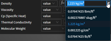
• Field level unit specification is improved to allow you to type the desired units inline with the value as well as offering a drop-down showing the equivalent value in the other valid units, as shown in Figure 2.2: Example Inline Unit Drop-down.

  Figure 2.2: Example Inline Unit Drop-down

  
  
  

• Mesh Interface creation is improved and simplified, as well as offering diagnostics to help inform you of the overlap which you can use to determine whether the interface is physically relevant. Refer to Accessing Mesh Interface Settings in the Fluent User's Guide for additional information.

• You can now review cell zone adjacency and do bulk renaming of cell zones in the Adjacency panel, opened from a right-click of the Cell Zone Conditions node in the Settings tree.

Beta Features

• There are also some exciting new enhancements available as beta features that you may be interested in trying out. Detailed documentation is in the Fluent 2026 R1 Beta Features Manual.

Fluent Icing

Fluent Icing allows you to easily conduct in-flight icing simulations within a dedicated Fluent Application Client environment. The following additional functionality has been added in this release.

• Constant roughness output for iced surfaces

  The beading roughness output option in the ice physical models section updated to provide a choice between constant roughness or beading as the output roughness height from ICE3D. Constant roughness option will output the user specified roughness height on the iced areas only.

• Water film reinjection with DPM (beta)

  Water film that accumulates at trailing edges or separation lines can now be released into the flow with the Lagrangian particle tracking model in the multi-shot and CHT workflows.

• Particle impingement update during CHT anti-icing with DPM (beta)

  The anti-icing simulations using Lagrangian tracking and impingement can now have the particle tracks reevaluated at each CHT loop, to recompute collection efficiency with changes in droplet splashing and bouncing and ice crystal sticking efficiency. This capability can also be coupled with DPM water film reinjection to represent water film shedding from heated surfaces.

  Changes to existing features and behavior

• DPM mixing plane

  Mixing plane implementation that transfers particles collected at the exit of an upstream turbomachinery row to the downstream row is updated for accuracy and robustness. Particles that arrive at the mixing plane outlets are collected in a high-resolution bin distribution with individual flow rate radial profiles. Vapor flow rate profile is included as a separate bin before the particle bins. The out.mpdat file that lists these radial profiles for each bin can be used to plot changes in radial flow rate distributions of bins as they move from one row to the next. Effects of physical phenomena like ice crystal shattering (if provided via UDF) can be observed as changes in particle size distribution and flow rates past rotors.

• ICE3D solution field profile macros for multishot UDFs

  Some ICE3D solution fields are now automatically extracted as Fluent boundary profile data which can be used as inputs for UDFs in the next shot in multi-shot workflows with UDF macros specifically assigned to these variables. This replaces the need to define UDMs and assign icing values to them at the completion of an ice run, simplifying the use of icing solution in particle/wall interaction UDFs that control splashing, bouncing, shattering, and sticking efficiency.

• Multishot runs

  • Multishot runs will no longer remesh the last shot and list the last shot + 1 entry in the project view. Calculations will stop with the final ice step. Users can continue the multishot resuming from the mesh update step of the last shot and increasing the number of shots. This avoids waiting for the last remeshing step when it is not needed.

  • The first shot’s mesh will not be loaded automatically when a multishot ends. This is done to keep the last shot’s volume solution fields in memory to allow post processing. When using very large grids, having to reload the last shot’s case and data files to post-process is costly. Now the last solution will be readily available at the end of the run.

  • To start a new multishot from the original grid, users MUST hit the Reset Multishot button to reload the original grid, as this is no longer done automatically. If there is a restart air solution to be provided, this has to be loaded manually as well after reloading the initial case file.

  • Custom multishot feature corrected, and the button to display the shot-by-shot settings is moved adjacent to the drop down menu. The only available parameter to vary in this version is the icing time per shot.

  • If remeshing fails during a multishot run, the last shot will be reloaded and restart step will be set to Mesh Update. Users can make changes in meshing settings like edge sizing, material point coordinates and wrap resolution factor to retry remeshing.

• De-icing CHT run memory management

  A defect with the FENSAP library was causing a cumulative memory leak in the multishot workflows, which resulted in de-icing simulations with many time steps and inner iterations to crash when the available memory is completely filled. The problem is corrected which extends the number of time steps de-icing simulations can run.

• DPM inlet velocity specification

  Lagrangian tracking can now assign air flow velocities to particle tracks at inlets. This is done by unchecking the velocity option on the inlet boundary panel for particles, as done similarly for the Eulerian (DROP3D) implementation.

Fluent Aero

Fluent Aero allows you to easily explore the aerodynamic performance of aircraft under a wide range of flight regimes, from subsonic to hypersonic conditions, all within a dedicated Fluent Application Client environment. A streamlined workflow guides you through the creation of a matrix of flight conditions or design points where single and multiple flight parameters, such as angle of attack, Mach number, altitude, etc., can vary. Most common models, solvers, and convergence settings of Fluent are tuned using the latest best practices for external aerodynamic problems and are available in Fluent Aero’s user interface. In this manner, simulations can be conducted in a quick and user-friendly environment. The full capabilities of the Fluent Solution workspace remain accessible when its session is displayed through Workspaces → Solution within the Fluent Aero ribbon. Tutorials are available to provide examples on how to conduct exploratory simulations using single and multiple flight parameters.

In this release, a broad range of features have been added and are described below.

• Mesh Adaption

  • A new combined Hessian Indicator has been introduced that uses Entropy (Combined Hessian - Entropy) instead of Turbulent Viscosity (Combined Hessian - Turbulence). This indicator has been identified as more generic and cost-effective when producing accurate RANS results during the High-Lift Workshop 5.

  • Extra wall monitors have been added to track average temperature and heat flux convergence during adaption cycles as appropriate for high-speed flow simulations.

  • It is now possible to Interrupt an adaption cycle and to directly continue to the next cycle or the next design point without losing the interrupted cycle data.

• Expansion of Unit Systems (Beta)

  • An additional unit system has been added to Fluent Aero, US Engineering Common. This new unit system is similar to the US Engineering system but with changes to the units representing angle, length and temperature quantities.

  • The latest unit system used in a simulation is automatically saved and reloaded between simulations.

• Overset Meshes for Parametric Analysis (Beta)

  • Geometric Parametric Analyses can be conducted using Overset Meshes in Fluent Aero. In this release, an aircraft component inside an overset mesh can be combined with a background mesh, that contains the aircraft, to conduct parametric simulations by varying the angular position of this component per design point. Therefore, it is now possible to study the impact of an aircraft component on the performance of the entire aircraft.

  • Multiple overset meshes can be supported in Fluent Aero-with or without mesh adaption per design point.

  • Geometric Parametric Analyses with Overset can be conducted using RANS and URANS in 2.5D and 3D simulations in Fluent Aero.

• Transient Calculations (Beta)

  • URANS calculations have been introduced in Fluent Aero to capture the natural transient flow behaviour of certain conditions per design point.

  • Convergence Criteria and Default or Robust Convergence Settings based on best practices have not been introduced and therefore these settings should be specified in the baseline case file.

  • Transient calculations can start from a previously steady state solution computed with or without mesh adaption in Fluent Aero.

  • Intermediate URANS solutions can be saved to post-process results.

  • Only instantaneous aerodynamic forces and moments are provided through tables and graphs of Fluent Aero. Time-averaged solutions are not provided.

  • Prescribed time-dependent sinusoidal oscillatory angular motions are supported at each overset aircraft component to study transient aerodynamic responses.

Polyflow

The Polyflow workspace is a means to explore manufacturing applications of highly viscous materials such as polymer extrusion, blowmolding, fiber spinning, etc. within the Fluent environment.

• Polyflow Workspace Add-In for Workbench

  Gives access to a complete workflow, geometry modelling to results analysis, in the Workbench environment.

• Statistical analysis

  Allows statistical analysis as in the Polystat tool of the Polyflow Classic. Relies on CFD-Post to create relevant animations.

• Adaptive meshing for large variations of field

  Allows to refine the mesh to limit the variation of specific fields on a finite element.

• Surface tension for 2D and 3D free surfaces

  Allows to include surface tension forces in flow modelling and dynamic contact point in 2D.

• Calibrator model

  Allows to simulate actual calibrators that shape and cool extrudate as well as conveyors that support profiles in extrusion lines.

• Mesh quality postprocessor (beta)

  Allows to display element quality metric when transient mesh deformation occurs, possibly with mesh adaption.

• Velocity imposed on a free surface (beta)

  Allows to prescribe the motion of a free surface via its velocity in transient simulations.

• Electrical heating (beta)

  Allows to calculate the electric potential field and its joule effect on the fluid temperature.

Mesh Generation

• When using the Rapid Octree mesher, the following improvements affect the code behavior:

  • The smooth mesh coarsening option is now enabled by default for the Rapid Octree mesher, so that the refined cells follow the geometry better. This option increases cell quality in most cases, and can reduce the overall cell count while maintaining a comparable level of accuracy. If you do not want to take advantage of this option, you can disable it by entering the following text command: mesh/rapid-octree/mesh-sizing/smooth-mesh-coarsening? no. (Mesh Parameters)

  • When you specify a reference size (in order to precisely set the edge length for the maximum cell size), the Rapid Octree mesher bounding box will now retain its extents better than in previous releases. Typically it will not be revised at all, and if it is revised, it will only undergo a slight change (up to the maximum cell size). For setups that use the Bound by Bounding Box or Selected Material Points for the Volume Specification, you should still verify that the bounding box is properly located after specifying the reference size. (Defining the Reference Size)

• In previous releases, reading a case file into the meshing mode of Ansys Fluent and then writing out a mesh file would store the original case file version number in the resulting mesh file. If this mesh file was used to set up simulations in later versions of the solver mode of Ansys Fluent, this could result in older solver defaults / behaviors being used unexpectedly.

  In release 2026 R1, this case file version information is omitted from any mesh file written by meshing mode. Note that this change does not affect meshes newly created from geometry in meshing mode, as case file version info was never present unless starting from a case file.

Solver-Meshing

• The following improvements are now available when fusing face zones:

  • The fusing performance is much faster, especially when fusing a large number of face zones.

  • When fusing multiple zones, the naming convention for the resulting zones is improved to be that of the first zone of each fused zone pair, which can help to identify and track the zones.

  • The information printed in the console during fusing is improved: unnecessary warnings are removed, more detailed information is provided (including the IDs of the fused zone pairs and the resulting zones), and a summary is included at the end that provides the number of zone pairs that were fused.

  For information about fusing face zones, see Fusing Selected Face Zones.

• When you perform a mesh check, additional checks are now performed to detect mesh degeneracy. You should repair the mesh if any degeneracies are found, as they may cause the solver to fail or may compromise the solver robustness. (Checking the Mesh)

Solver-Numerics

• Minor inconsistencies are now corrected in the wall distance calculation (when using the default geometric method) for double-precision cases.

Cell Zones and Boundary Conditions

• Fluent now has an improved method for handling name conflicts for cell zones and boundary zones. A name conflict arises when a new zone is created (by actions such as copying a cell zone, appending a case file, and so on) and the name initially generated with the default convention is already used by an existing zone, and so the proposed zone name must be modified. The new handling for name conflicts produces names that have improved consistency and readability, and may be more intuitive for wall-shadow pairs. Note that while the names for new zones may differ compared to those generated in previous releases, the IDs will remain the same.

  For example, one of the changes in handling name conflicts can be seen in the following: if you were to repeatedly append the same case file with a cell zone named fluid using the previous release, you would end up with cell zones named fluid.1, fluid.1.1, and fluid.1.1.1, whereas in the current release those same zones would be named fluid.1, fluid.2, and fluid.3, respectively.

Multiphase Models, DDPM Models

• The solution results may now be more accurate for granular multiphase cases that involve the filtered drag model in the Euler/Euler model and the DDPM model on coarse meshes due to a correction of the terminal velocity calculations.

• For cases that use the incompatible combination of the alternative energy treatment for interphase mass transfer and real gas property (RGP) tables, the default sensible enthalpy formulation will be used instead of the alternative formulation. Consequently, you may notice changes in solution results, as the default formulation properly accounts for the heat source due to mass transfer.

Fluent Native GPU Solver

• The default group size for the coupled linear solver is now reduced from 8 to 4, in order to improve the robustness of the coupled linear solver. To revert this change, enter the following Scheme command in the console: (rpsetvar 'gpuapp/amg-coupled/group-size 4).

• When using the pressure-based solver with a segregated scheme for the pressure-velocity coupling, the linear solver now respects the cycle type that you have specified for pressure. This is used primarily for some reacting flow workflows where this setting is set explicitly to enhance robustness. To revert this change, set the pressure cycle type to its default setting of V-Cycle (for example, in the Multigrid tab of the Advanced Solution Controls dialog box).

• At porous interfaces, pressure is now extrapolated in the normal direction only, in order to improve robustness issues at fluid-porous interfaces with skewed meshes. There is no way to revert this improvement.

• For compressible transient flows that use the pressure-based solver with a segregated scheme for the pressure-velocity coupling, the solver now uses the pressure relaxation factor for the compressible transient linearization to give faster convergence within a time step, and for consistency with the CPU solver. To revert this change, enter the following Scheme command in the console: (gpuapp-set-bool “flow/full-transient-compressible-pressure-relaxation" #t).

• For LES / SBES simulations, the discretization of normal stress at walls and of the velocity gradients used to compute the turbulent viscosity have been modified to improve robustness. To revert this change, enter each of the following Scheme commands in the console:

  • (gpuapp-set-string "turbulence/normal-stress-option-at-walls" "turbulent")

  • (gpuapp-set-bool "turbulence/use-lsq-grad-for-turbulent-viscosity" #f)

Graphics, Reporting, and Postprocessing

• The iso-surface and iso-clip algorithm is improved:

  • For iso-surfaces, it offers improved performance, particularly when creating multiple surfaces at once. It also has improved handling of boundaries during surface creation. Note that there may be some differences when comparing with previous releases. In particular, minor changes in appearance may occur when all edges are displayed. Faceting may also be slightly different.

  • For iso-clips, faceting is improved. Note that there may be a noticeable change in the facet count or in edge displays.

  Use the surface/settings/previous-defaults/pre-26.1-algorithm text command to revert to the earlier algorithm.

Polyflow

• • The number of processors used by the workspace solver has been increased from 2 to 4 processors.

  • Mesh objects created by the workspace no longer use generic naming conventions (mesh-1, mesh-2, etc.) by default. The new default is to use the topological names found in the mesh file. The behavior can be changed using Preferences. See Setting Preferences for Polyflow in the Fluent Workspaces User's Guide for details.