


SHELL229
4-Node Coupled-field Shell
SHELL229 Element Description
SHELL229 is a 3D layered shell element having in-plane thermal and electrical capabilities (membrane behavior), as well as structural capability (membrane and bending behavior). It supports the following physics combinations:
Structural-Thermal
Thermal-Electric
Structural-Thermoelectric
The element has four nodes with no limitation on the number of material layers (defined by the SECDATA command). It has up to 8 degrees of freedom at each node, including temperature and voltage in membrane format, as well as translation and rotation in 3D corresponding to structural analysis. The temperature generated by SHELL229 can be passed to structural shell elements (SHELL181 or SHELL281) in order to model thermal strain. See SHELL229 in the Mechanical APDL Theory Reference for more details about this element. For verification examples, see VM174, VM215, and VM223.
Figure 229.1: SHELL229 Geometry
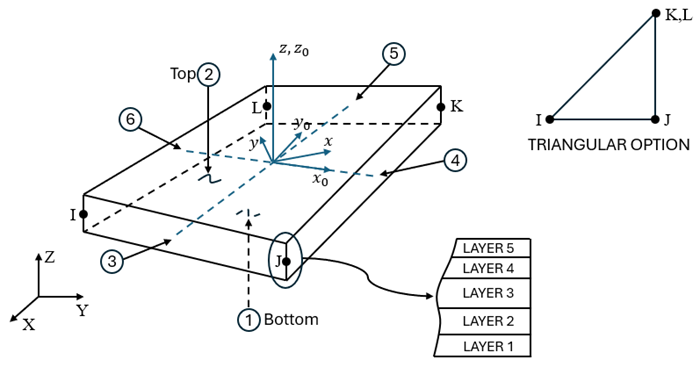
xo = element x-axis if ESYS is not supplied.
x = element x-axis if ESYS is supplied.
SHELL229 Input Data
The geometry, node locations, and coordinates systems for this element are shown in Figure 229.1: SHELL229 Geometry. The element is defined by four nodes, one thickness per layer, a material angle for each layer, and the material properties.
The cross-sectional properties are input using the SECTYPE,,SHELL and SECDATA commands. These properties are the thickness, material number, and orientation of each layer. The number of integration points through the thickness is always 1, irrespective of the number entered in the SECDATA command. Real constants are not used for this element.
The default orientation for this element has the S1 (shell surface coordinate) axis aligned with the element's first parametric direction at its center.
The default first surface direction S1 can be reoriented in the element reference plane (as
shown in Figure 229.1: SHELL229 Geometry) using the ESYS command. You
can further rotate S1 by angle THETA (in degrees) for each layer via
the SECDATA command to create layer-wise coordinate systems. See Coordinate Systems for details.
KEYOPT(1) determines the element degree-of-freedom (DOF) set and the corresponding force labels and reaction solution. KEYOPT(1) is set equal to the sum of the field keys shown in Table 229.1: SHELL229 Field Keys. For example, set KEYOPT(1) = 110 for a thermal-electric analysis (thermal field key + electric field key = 10 + 100). This activates a thermal-electric analysis with TEMP and VOLT as DOF labels and heat flow and electric current as reaction solutions.
The coupled-field analysis KEYOPT(1) settings, DOF labels, force labels, reaction solutions, and analysis types are shown in the following table.
Table 229.2: SHELL229 Coupled-Field Analysis
| Coupled-Field Analysis | KEYOPT(1) | DOF Label | Force Label | Reaction Solution | Analysis Type |
|---|---|---|---|---|---|
| Structural-Thermal | 11 | UX, UY, UZ, ROTX, ROTY, ROTZ, TEMP | FX, FY, FZ, MX, MY, MZ, HEAT | Force, Heat Flow | Static, Full Transient |
| Thermal-Electric | 110 | TEMP, VOLT | HEAT, AMPS | Heat Flow, Electric Current | Static, Full Transient |
| Structural-Thermoelectric | 111 | UX, UY, UZ, ROTX, ROTY, ROTZ, TEMP, VOLT | FX, FY, FZ, MX, MY, MZ, HEAT, AMPS | Force, Heat Flow, Electric Current | Static, Full Transient |
As shown in the following table, material property requirements consist of those required for the individual fields (structural, thermal, and electric conduction) and those required for field coupling. Individual material properties are defined using the MP and MPDATA commands. Nonlinear and multiphysics material models are defined using the TB command.
Table 229.3: Structural Material Properties
| Field | Field Key | Material Properties and Material Models |
|---|---|---|
| Structural | 1 | EX, EY, EZ, PRXY, PRYZ, PRXZ (or NUXY, NUYZ, NUXZ), GXY, GYZ, GXZ, DENS, ALPD, BETD, DMPR, DMPS ALPX, ALPY, ALPZ (or CTEX, CTEY, CTEZ, or THSX, THSY, THSZ), REFT –- Anisotropic hyperelasticity, Anisotropic elasticity, Bergstrom-Boyce, Chaboche nonlinear kinematic hardening, Creep, Elasticity, Hill anisotropy, Hyperelasticity, Mullins effect, Voce isotropic hardening law, Plasticity, Prony series constants for viscoelastic materials, Rate-dependent plasticity (viscoplasticity), Rate-independent plasticity, Material-dependent alpha and beta damping (Rayleigh damping), Material-dependent structural damping, Shift function for viscoelastic materials |
Table 229.4: SHELL229 Material Properties and Material Models
| Coupled-Field Analysis | KEYOPT(1) | Material Properties and Material Models | |
|---|---|---|---|
| Structural-Thermal | 11 | Structural | See Table 229.3: Structural Material Properties |
| Thermal | KXX, KYY, C, DENS, ENTH, HF | ||
| Coupling | ALPX, ALPY, ALPZ, REFT, QRATE | ||
| Thermal-Electric | 110 | Thermal | KXX, KYY, DENS, C, ENTH, HF |
| Electric | RSVX, RSVY | ||
| Coupling | –- | ||
| Structural-Thermoelectric | 111 | Structural | See Table 229.3: Structural Material Properties |
| Thermal | KXX, KYY, C, DENS, ENTH, HF | ||
| Electric | RSVX, RSVY | ||
| Coupling | ALPX, ALPY, ALPZ, REFT, QRATE | ||
The density, thermal conductivity, specific heat, and electrical resistivity can all be defined either with the MP command or the TB command.
The electrical resistivity can be defined as a function of primary variables by using tabular input on the MP command. For more information, see Defining Linear Material Properties Using Tabular Input in the Material Reference. Alternatively, TB,ELEC can be used to define electrical resistivity with TBOPT = RSV or electrical conductivity with TBOPT = COND. For more information, see Anisotropic Electrical Conductivity.
Nodal loads are defined with the D and F commands.
Element loads are described in Element Loading. Loads may be input on the element faces indicated by the circled numbers in Figure 229.1: SHELL229 Geometry using the SFE command. Body loads may be input at the element's material layers using the BFE commands.
SHELL229 surface and body loads are given in the following table. Most surface and body loads can be defined as a function of primary variables by using tabular input. For more information, see Applying Loads Using Tabular Input in the Basic Analysis Guide and the individual surface or body load command description in the Command Reference.
Table 229.5: SHELL229 Surface and Body Loads
| Coupled-Field Analysis | KEYOPT(1) | Load Type | Load | Command Label |
|---|---|---|---|---|
| Structural-Thermal | 11 | Surface | Pressure | PRES |
| Convection Heat Flux Radiation | CONV HFLUX RDSF | |||
| Body | Heat generation on material layers HG(1), HG(2), . . . , HG(number of layers) | HGEN | ||
| Thermal-Electric | 110 | Surface | Convection Heat Flux Radiation | CONV HFLUX RDSF |
| Body | Heat generation on material layers HG(1), HG(2), . . . , HG(number of layers) | HGEN | ||
| Structural-Thermoelectric | 111 | Surface | Pressure | PRES |
| Convection Heat Flux Radiation | CONV HFLUX RDSF | |||
| Body | Heat generation on material layers HG(1), HG(2), . . . , HG(number of layers) | HGEN |
The surface loads are input on a per-unit-area basis at all six faces including the shell edges:
Face 1 (I-J-K-L) (bottom, -z side)
Face 2 (I-J-K-L) (top, +z side)
Face 3 (J-I)
Face 4 (K-J)
Face 5 (L-K)
Face 6 (I-L)
This is in contrast to SHELL157 and SHELL181 where surface loads on shell edges (faces 3 to 6 above) are input on a per-unit-length basis.
The thermal surface loads, including radiation, convection, and heat flux can only be defined by the SFE command. Use the surface effect element SURF152 to generate film coefficients and bulk temperatures. SURF152 can also be used with FLUID116.
Element body loads may be input on a per layer basis. They can be defined with the BFE command only. One body load value is applied to the entire layer. If the first layer body load is input, and all others are unspecified, they default to the value specified for the first layer.
The body loads can be applied on material layers, where HG(1), HG(2), HG(3), . . . ., HG (number of material layers) can be defined with the BFE command only.
A summary of the element input is given in "SHELL229 Input Summary". A general description of element input is given in Element Input.
SHELL229 Input Summary
- Nodes
I, J, K, L
- Degrees of Freedom
Set by KEYOPT(1). See Table 229.2: SHELL229 Coupled-Field Analysis. - Material Properties
- Surface Loads
- Body Loads
- Special Features
- KEYOPT(1)
Element degrees of freedom. See Table 229.2: SHELL229 Coupled-Field Analysis. - KEYOPT(2)
Coupling method between the DOFs:
- 0 --
Strong (matrix) coupling. May produce an unsymmetric matrix. In a linear analysis, a coupled response is achieved after one iteration.
- 1 --
Weak (load vector) coupling. Produces a symmetric matrix and requires at least two iterations to achieve a coupled response.
- KEYOPT(3)
Element stiffness for structural field:
- 0 --
Bending and membrane stiffness (default).
- 1 --
Membrane stiffness only.
- KEYOPT(4)
Integration option for structural field:
- 0 --
Reduced integration with hourglass control (default).
- 2 --
Full integration with incompatible modes.
Note: This keyoption is primarily used in structural analysis. However, for the degenerate triangular shape, the number of integration points in thermal and electrical analyses increases from 1 to 3 by changing KEYOPT(4) from 0 to 2.
- KEYOPT(7)
Evaluation of film coefficient:
- 0 --
Evaluate film coefficient (if any) at average film temperature, (TS+TB)/2.
- 1 --
Evaluate at element surface temperature, TS.
- 2 --
Evaluate at fluid bulk temperature, TB.
- 3 --
Evaluate at differential temperature, |TS-TB|.
- KEYOPT(8)
Material layer data storage:
- 0 --
Store data for bottom of bottom layer and top of top layer (default).
- 1 --
Store top and bottom data for all layers (the volume of data may be considerable).
- KEYOPT(9)
Thermoelastic damping (piezocaloric effect) in coupled-field transient analysis having structural and thermal degrees of freedom:
- 0 --
Active. Evaluated at the reference temperature.
- 1 --
Suppressed (required for frictional heating analyses).
- 2 --
Active. Evaluated at the actual temperature.
- KEYOPT(13)
Film coefficient matrix:
- 0 --
The program determines whether to use a diagonal or consistent film coefficient matrix (default).
- 1 --
Use a diagonal film coefficient matrix.
- 2 --
Use a consistent film coefficient matrix.
- KEYOPT(15)
Specific heat matrix:
- 0 --
The program determines whether to use a diagonal or consistent specific heat matrix (default).
- 1 --
Use a diagonal specific heat matrix.
- 2 --
Use a consistent specific heat matrix.
SHELL229 Output Data
The solution output associated with the element is in two forms:
Nodal degrees of freedom included in the overall nodal solution
Additional element output shown in Table 229.6: SHELL229 Element Output Definitions
Output temperatures may be read by structural shell elements SHELL181 and SHELL281 via the LDREAD,TEMP command.
Convection heat flux is positive out of the element. Applied heat flux is positive into the element.
The element output directions are parallel to the layer coordinate system.
A general description of solution output is given in Solution Output. See the Basic Analysis Guide for ways to view results.
To see the distribution of element quantities through the thickness for this element, enter the POST1 postprocessor (/POST1), then issue /GRAPHICS,POWER and /ESHAPE,1 followed by PLESOL.
The Element Output Definitions table uses the following notation:
A colon (:) in the Name column indicates that the item can be accessed by the Component Name method (ETABLE, ESOL). The O column indicates the availability of the items in the file jobname.out. The R column indicates the availability of the items in the results file.
In either the O or R columns, “Y” indicates that the item is always available, a letter or number refers to a table footnote that describes when the item is conditionally available, and “-” indicates that the item is not available.
Table 229.6: SHELL229 Element Output Definitions
| Name | Definition | O | R |
|---|---|---|---|
| ALL ANALYSES | |||
| EL | Element number | - | Y |
| NODES | Nodes - I, J, K, L | - | Y |
| MAT | Material number | - | Y |
| THICK | Shell thickness | - | Y |
| VOLU: | Volume | - | Y |
| XC, YC, ZC | Location where results are reported | - | [a] |
| ALL ANALYSES WITH A STRUCTURAL FIELD | |||
| PRES | Pressures P1 at nodes I, J, K, L; P2 at I, J, K, L; P3 at J,I; P4 at K,J; P5 at L,K; P6 at I,L | - | Y |
| LOC | TOP, MID, BOT, or integration point location | - | [b] |
| S:X, Y, Z, XY, YZ, XZ | Stresses | [c] | [d] |
| S:1, 2, 3 | Principal stresses | - | [d] |
| S:INT | Stress intensity | - | [d] |
| S:EQV | Equivalent stress | - | [d] |
| EPEL:X, Y, Z, XY | Elastic strains | [c] | [d] |
| EPEL:EQV | Equivalent elastic strains[e] | - | [d] |
| EPTH:X, Y, Z, XY | Thermal strains | [c] | [d] |
| EPTH:EQV | Equivalent thermal strains [e] | - | [d] |
| EPPL:X, Y, Z, XY | Average plastic strains | [c] | [f] |
| EPPL:EQV | Equivalent plastic strains [e] | - | [f] |
| EPCR:X, Y, Z, XY | Average creep strains | [c] | [f] |
| EPCR:EQV | Equivalent creep strains [e] | - | [f] |
| EPTO:X, Y, Z, XY | Total mechanical strains (EPEL + EPPL + EPCR) | [c] | - |
| EPTO:EQV | Total equivalent mechanical strains (EPEL + EPPL + EPCR) | - | - |
| NL:SEPL | Plastic yield stress | - | [f] |
| NL:EPEQ | Accumulated equivalent plastic strain | - | [f] |
| NL:CREQ | Accumulated equivalent creep strain | - | [f] |
| NL:SRAT | Plastic yielding (1 = actively yielding, 0 = not yielding) | - | [f] |
| NL:PLWK | Plastic work/volume | - | [f] |
| NL:HPRES | Hydrostatic pressure | - | [f] |
| SEND:ELASTIC, PLASTIC, CREEP, ENTO | Strain energy densities | - | [f] |
| N11, N22, N12 | In-plane forces (per unit length) | - | Y |
| M11, M22, M12 | Out-of-plane moments (per unit length) | - | [g] |
| Q13, Q23 | Transverse shear forces (per unit length) | - | [g] |
| ε11, ε22, ε12 | Membrane strains | - | Y |
| k11, k22, k12 | Curvatures | - | [g] |
| γ13, γ23 | Transverse shear strains | - | [g] |
| ILSXZ | SXZ interlaminar shear stress | - | Y |
| ILSYZ | SYZ interlaminar shear stress | - | Y |
| ILSUM | Magnitude of the interlaminar shear stress vector | - | Y |
| ILANG | Angle of interlaminar shear stress vector (measured from the element x axis toward the element y axis in degrees) | - | Y |
| Sm: 11, 22, 12 | Membrane stresses | - | Y |
| Sb: 11, 22, 12 | Bending stresses | - | Y |
| Sp: 11, 22, 12 | Peak stresses | - | Y |
| St: 13, 23 | Averaged transverse shear stresses | - | Y |
| ALL ANALYSES WITH A THERMAL FIELD | |||
| AREA | Face area | 1 | 1 |
| HFAVG | Average film coefficient of the face | - | 1 |
| TAVG | Average face temperature | 1 | 1 |
| TBAVG | Average bulk temperature | 1 | - |
| HEAT RATE | Heat flow rate across face by convection | 1 | 1 |
| HFLXAVG | Heat flow rate per unit area across face caused by input heat flux | - | 1 |
| ADDITIONAL OUTPUT FOR STRUCTURAL-THERMAL ANALYSIS (KEYOPT(1) = 11) | |||
| TG: X, Y, Z, SUM | Thermal gradient components and vector magnitude | - | [b] |
| TF: X, Y, Z, SUM | Thermal flux components and vector magnitude | - | [b] |
| PHEAT | Plastic heat generation rate per unit volume | - | [b] |
| VHEAT | Viscoelastic heat generation rate per unit volume | - | [b] |
| ADDITIONAL OUTPUT FOR THERMAL-ELECTRIC ANALYSIS (KEYOPT(1) = 110) | |||
| TG:X, Y, Z, SUM | Thermal gradient components and vector magnitude | - | [b] |
| TF:X, Y, Z, SUM | Thermal flux components and vector magnitude | - | [b] |
| EF: X, Y, Z, SUM | Electric field components and vector magnitude | - | [b] |
| JC: X, Y, Z, SUM | Conduction current density components and vector magnitude | - | [b] |
| JS: X, Y, Z, SUM | Current density components (in the global Cartesian coordinate system) and vector magnitude | - | [b] |
| JHEAT | Joule heat generation per unit volume | - | [b] |
| ADDITIONAL OUTPUT FOR STRUCTURAL-THERMOELECTRIC ANALYSIS (KEYOPT(1) = 111) | |||
| TG:X, Y, Z, SUM | Thermal flux components and vector magnitude | - | [b] |
| TF:X, Y, Z, SUM | Thermal flux components and vector magnitude | - | [b] |
| EF: X, Y, Z, SUM | Electric field components and vector magnitude | - | [b] |
| JC: X, Y, Z, SUM | Conduction current density components and vector magnitude | - | [b] |
| JS: X, Y, Z, SUM | Current density components (in the global Cartesian coordinate system) and vector magnitude | - | [b] |
| JHEAT | Joule heat generation per unit volume | - | [b] |
| PHEAT | Plastic heat generation rate per unit volume | - | [b] |
| VHEAT | Viscoelastic heat generation rate per unit volume | - | [b] |
[b] Solution values are output only if calculated (based on input values).
[c] Stresses, total strains, plastic strains, elastic strains, creep strains, and thermal strains in the element coordinate system are available for output (at all section points through thickness). If layers are in use, the results are in the layer coordinate system.
[d] The following stress solution repeats for top, middle, and bottom surfaces.
[e] The equivalent strains use an effective Poisson's ratio: for elastic and thermal this value is set by the user (MP,PRXY). For plastic and creep, this value is set at 0.5.
[f] Nonlinear solution output for top, middle, and bottom surfaces, if the element has a nonlinear material, or if large-deflection effects are enabled (NLGEOM,ON) for SEND.
[g] Not available for KEYOPT(3) = 1 (membrane only).
Table 229.6: SHELL229 Element Output Definitions lists output available through the ETABLE command using NMISC item. See Element Table for Variables Identified By Sequence Number in the Basic Analysis Guide and The Item and Sequence Number Table in this reference for more information. The following notation is used in Table 229.7: SHELL229 Item and Sequence Numbers:
- Name
Output quantity as defined in Table 229.6: SHELL229 Element Output Definitions
- Item
Predetermined item label for ETABLE command
- FCn
Sequence number for solution items for element Face n
Table 229.8: SHELL229 SMISC Item and Sequence Numbers lists output available through the ETABLE command using SMISC item for all analyses with a structural field. See Creating an Element Table and The Item and Sequence Number Table in this reference for more information. The following notation is used:
- Name
Output quantity as defined in the Table 181.1: SHELL181 Element Output Definitions
- Item
Predetermined Item label for ETABLE
- E
Sequence number for single-valued or constant element data
- I,J,K,L
Sequence number for data at nodes I, J, K, L
Table 229.8: SHELL229 SMISC Item and Sequence Numbers
| Output Quantity Name | ETABLE and ESOL Command Input | |||||
|---|---|---|---|---|---|---|
| Item | E | I | J | K | L | |
| N11 | SMISC | 1 | - | - | - | - |
| N22 | SMISC | 2 | - | - | - | - |
| N12 | SMISC | 3 | - | - | - | - |
| M11 | SMISC | 4 | - | - | - | - |
| M22 | SMISC | 5 | - | - | - | - |
| M12 | SMISC | 6 | - | - | - | - |
| Q13 | SMISC | 7 | - | - | - | - |
| Q23 | SMISC | 8 | - | - | - | - |
| ε11 | SMISC | 9 | - | - | - | - |
| ε22 | SMISC | 10 | - | - | - | - |
| ε12 | SMISC | 11 | - | - | - | - |
| k11 | SMISC | 12 | - | - | - | - |
| k22 | SMISC | 13 | - | - | - | - |
| k12 | SMISC | 14 | - | - | - | - |
| γ13 | SMISC | 15 | - | - | - | - |
| γ23 | SMISC | 16 | - | - | - | - |
| P1 | SMISC | - | 18 | 19 | 20 | 21 |
| P2 | SMISC | - | 22 | 23 | 24 | 25 |
| P3 | SMISC | - | 27 | 26 | - | - |
| P4 | SMISC | - | - | 29 | 28 | - |
| P5 | SMISC | - | - | - | 31 | 30 |
| P6 | SMISC | - | 32 | - | - | 33 |
| Sm: 11 | SMISC | 34 | - | - | - | - |
| Sm: 22 | SMISC | 35 | - | - | - | - |
| Sm: 12 | SMISC | 36 | - | - | - | - |
| Sb: 11 | SMISC | 37 | - | - | - | - |
| Sb: 22 | SMISC | 38 | - | - | - | - |
| Sb: 12 | SMISC | 39 | - | - | - | - |
| Sp: 11 (at shell bottom) | SMISC | 40 | - | - | - | - |
| Sp: 22 (at shell bottom) | SMISC | 41 | - | - | - | - |
| Sp: 12 (at shell bottom) | SMISC | 42 | - | - | - | - |
| Sp: 11 (at shell top) | SMISC | 43 | - | - | - | - |
| Sp: 22 (at shell top) | SMISC | 44 | - | - | - | - |
| Sp: 12 (at shell top) | SMISC | 45 | - | - | - | - |
| St: 13 | SMISC | 46 | - | - | - | - |
| St: 23 | SMISC | 47 | - | - | - | - |
SHELL229 Assumptions and Restrictions
Zero thickness layers are not allowed.
The tabular thickness specified by SECFUNCTION is not supported.
The mass transport is not supported.
Nonlinear material properties are evaluated at each integration point.
This element may not be compatible with other elements with the VOLT degree of freedom. To be compatible, the elements must have the same reaction solution for the VOLT DOF. For more information, see Element Compatibility in the Low-Frequency Electromagnetic Analysis Guide.
Source current density, JS, and Joule heat, JHEAT, are available as both element and layer average values if KEYOPT(8) = 1, and only as element average values if KEYOPT(8) = 0. The layer average values can be accessed in /POST1 by issuing the LAYER command, and in /POST26 by issuing the LAYERP26 command. If either LAYER,0 or LAYERP26,0 is issued, then the element average value is printed.
The full quadrilateral shape provides higher accuracy compared to triangular shape. If possible, avoid the triangular shape, especially in areas with high stress gradients.
Setting KEYOPT(4) = 2 is recommended to better capture the stress gradients.
The section definition permits use of hyperelastic material models and elastoplastic material models in laminate definition. However, the accuracy of the solution is primarily governed by fundamental assumptions of shell theory. The applicability of shell theory in such cases is best understood by using a comparable solid model.
The layer orientation angle has no effect if the material of the layer is hyperelastic.
The through-thickness stress, SZ, is always zero.
If a shell section has a single layer and only one integration point, or if KEYOPT(3) = 1, the shell has no bending stiffness. This condition can cause solver and convergence problems.
Mass transport is not supported.
Nonlinear material properties are typically evaluated at each integration point, except for triangular shape with KEYOPT(4)=2, where structural material properties are evaluated at the centroid.