

This example presents the modal analysis of a rotating bladed disk.
The following example [Ruffini et al.] describes a modal analysis of the cyclically-symmetric bladed disk shown in Figure 5.24: Bladed Disk Geometry and Mesh. It is subjected to various rotational velocities (OMEGA). The prestress due to the centrifugal forces and the Coriolis forces are accounted for through the two-step linear perturbation analysis (PERTURB). Coriolis effects are activated (CORIOLIS). A modal analysis is then performed with the DAMP eigensolver (MODOPT).
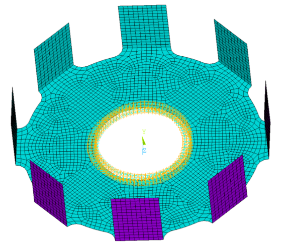
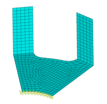
The structure is a disk composed of 8 blades and is clamped along its inner radius. It is cyclically symmetric and can be divided into 8 sectors. Only one sector, shown in Figure 5.25: Sector Mesh, is defined and meshed.
The Coriolis effects modify the natural frequencies when the rotational velocity increases from 0 to 500 RPM. In particular, the typical cyclic structure mode pairs undergo a frequency split: one frequency increases with rotational velocity (forward mode) while the other decreases (backward mode).
Ruffini, V., Schwingshackl, C., Green, J. Experimental and Analytical Study of Coriolis Effects in Bladed Disk. ASME. 2015.
The problem specifications are as follows:
Disk Dimensions
Outer Diameter: 200 mm
Inner Diameter: 80 mm
Thickness: 2 mm
Blade Dimensions
Height: 54 mm
Width: 40 mm
Material Properties
Young's Modulus: 191 GPa
Poisson's Ratio: 0.3
Density: 7850 kg/m3
The geometry, material, and mesh for the sector illustrated in Figure 5.25: Sector Mesh have been specified and saved in the input file, meshSector45.inp, which can be downloaded along with the entire input (input_cyclicExample08.dat) at this link: input_cyclicExample08.zip. You can use thess input files to model the example problem described.
/filname,cyclicCoriolis

/prep7

! input the mesh and material
/input,meshSector45,inp

! apply boundary conditions
cmsel,s,_FIXEDSU
d,all,all ! clamp along inner radius
nsel,all

! activate cyclic symmetry
cyclic

! create spin velocities
pi=acos(-1)
rpmToRad=pi/30

! define three velocities to investigate
*DIM,spin,,3
spin(1)=0
spin(2)=250*rpmToRad
spin(3)=500*rpmToRad

! array for storing modal frequencies at the above velocities
*DIM,freqCyc,,8,3

! define the modal step indices to extract
*DIM,stepIndI,,8
stepIndI(1)=1,2,2,3,3,4,4,5

*DIM,stepIndJ,,8
stepIndJ(1)=1,1,3,1,3,1,3,1

finish

allsel

*DO,I,1,3
    ! perform static analysis with coriolis effects (prestress/linear perturbation)
    /solu
    antype,static
    coriolis,on
    omega,0,spin(I),0
    rescontrol,linear,all,1
    ! do not use master-slave relationship between boundary nodes
    cycopt,msup,no
    solve
    finish

    ! perform modal analysis
    /solu
    antype,static,restart,,,perturb
    perturb,modal
    solve,elform

    modopt,damp,16
    mxpand,all
    solve
    finish

    /post1
    file,cyclicCoriolis,rstp

    *DO,J,1,8
        indI=stepIndI(J)
        indJ=stepIndJ(J)
        set,indI,indJ,,imag
        *get,freqCyc(J,I),active,,set,freq
    *ENDDO

    finish
*ENDDO

/com =============================
/com  Results for cyclic analysis
/com =============================
/com
/com Campbell diagram: natural frequencies vs. rotational velocities
/com
/com Velocity (RPM): 0         ; 250         ; 500
/com ND0:            %freqCyc(1,1)% ; %freqCyc(1,2)% ; %freqCyc(1,3)%
/com ND1 backward:   %freqCyc(2,1)% ; %freqCyc(2,2)% ; %freqCyc(2,3)%
/com ND1 forward:    %freqCyc(3,1)% ; %freqCyc(3,2)% ; %freqCyc(3,3)%
/com ND2 backward:   %freqCyc(4,1)% ; %freqCyc(4,2)% ; %freqCyc(4,3)%
/com ND2 forward:    %freqCyc(5,1)% ; %freqCyc(5,2)% ; %freqCyc(5,3)%
/com ND3 backward:   %freqCyc(6,1)% ; %freqCyc(6,2)% ; %freqCyc(6,3)%
/com ND3 forward:    %freqCyc(7,1)% ; %freqCyc(7,2)% ; %freqCyc(7,3)%
/com ND4:            %freqCyc(8,1)% ; %freqCyc(8,2)% ; %freqCyc(8,3)%
/com
/com =================================================================
The results of your analysis should match those shown below.
Table 5.3: Campbell Diagram: Natural Frequencies (Hz) vs. Rotational Velocities
| Rotational Velocity (RPM) | 0 | 250 | 500 |
|---|---|---|---|
| NDO | 186.629773 | 186.662264 | 186.75967 |
| ND1 Backward | 184.519563 | 183.735482 | 183.025736 |
| ND1 Forward | 184.519563 | 185.378438 | 186.312419 |
| ND2 Backward | 200.807987 | 199.264576 | 197.800111 |
| ND2 Forward | 200.807987 | 202.431166 | 204.134791 |
| ND3 Backward | 259.730415 | 257.461876 | 255.237401 |
| ND3 Forward | 259.730415 | 262.041871 | 264.394644 |
| ND4 | 308.632478 | 308.478103 | 308.020409 |