Introduce some basic methods for analyzing a simulation after it has been processed.
The purpose of this tutorial is to introduce some basic methods for analyzing a simulation after you have processed it. We will continue from where we left off in Part A.
You will learn how to:
Create Custom Properties
Visualize Custom Properties in a 3D View Window
Edit Color Scales
Create Time Plots
Track SPH elements with Tagging Calculations
Measure a surface mass flow rate
And you will use these features:
Time plot
Cube User Process
Tagging Calculation
Color Scales
If you completed Part A of this tutorial, ensure that FreeFlow project is open (Part B will continue from where Part A left off).
Download the
freeflow_tut02_files.zipfile here .Unzip
freeflow_tut02_files.zipto your working directory.Open FreeFlow 2026 R1.
Important: To make use of the FreeFlow project file provided, you must have FreeFlow 2026 R1 or later. If you have an earlier version of FreeFlow, please upgrade to the latest version, or complete Part A from scratch.
From the FreeFlow program, click the Open Project button, find the
freeflow_tut02_filesfolder, and then from thetutorial_02_A_pre-processingfolder, open thetutorial_02_pre-processing.freeflowfile.
Process the simulation (from the Simulation toolbar, click the Start button).
Now that the project has completed processing, we can begin to analyze it.
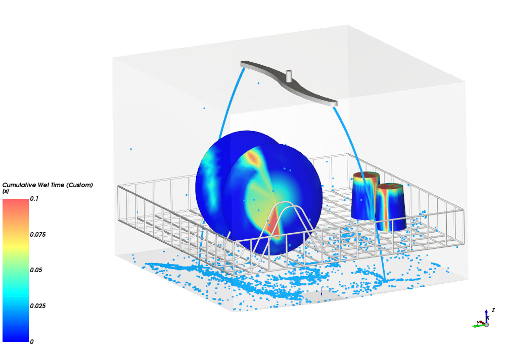
We want to check if the dishes are being washed, so we can analyze which parts of each dish are getting in contact with water and for how long.
To do that, we will create a Cumulative Wet Time property to see how different regions of the dishes interact with water.
Tip: The Cumulative Wet Time will calculate the total time that each geometry triangle got in contact with water.
To create this custom property, follow the steps below.
From Data panel, select plate_01 or any other dish component.
On the Data Editors panel, go to Properties tab and click the Add new custom property button.
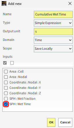
From the Add new dialog box, define the Name, Output unit and select SPH : Wet Time for Inputs, and click OK.
In the Custom Property dialog box, enter the Expression as follows and click OK.
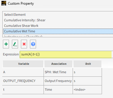
Note: This is a pythonic expression that gets the sum of the SPH : Wet Time for the whole simulation duration.
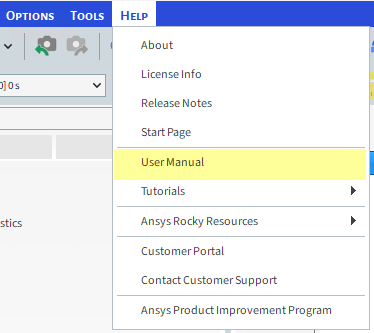
To learn more about this property, access the SPH Technical Manual (from the Menu | Help | Manuals).
COLORING THE 3D VIEW BY THE CUMULATIVE WET TIME
Now that the custom property is created, we are able to color the dishes by the Cumulative Wet Time. With a 3D View opened, follow the steps below.
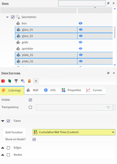
From the Data panel, multi-select the plate_01, plate_02, glass_01 and glass_02 geometries.
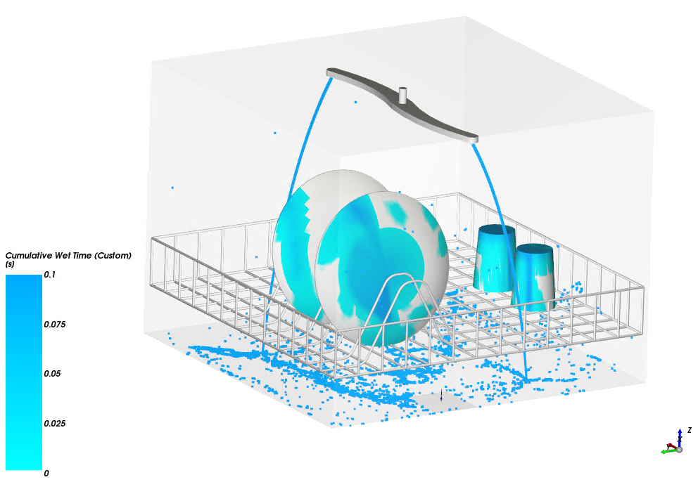
From the Data Editors panel, go to Colorings tab, ensure that Faces checkbox is enabled, and select Cumulative Wet Time (Custom) from the Grid-function drop-down list.
Move the slider on the time toolbar through different output times to see how the dishes are interacting with the water.
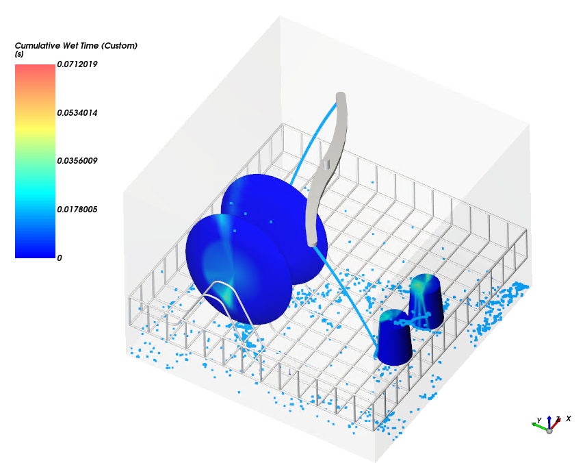
Note: Because the glasses have more surface area in contact with water than the plates, the cumulative wet time visualization needs a scale limits adjustment.
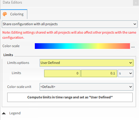
You may adjust the Cumulative Wet Time Color Scale in order to better visualize the fluid effect on the dishes regions.
From the Data panel, under Color Scales, select the Cumulative Wet Time (Custom) entity.
From the Data Editors panel, define the Limits options as User Defined and the Limits as follows.
With the 3D View opened, go to the last output time and check the cumulative wet time on the dishes for 5 seconds of operational time.
COLOR SCALE CONFIGURATION
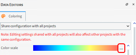
You can also change the colors of the Color-scale. If you want to export a customized animation (refer to Tutorial 01 on how to create an animation) with the wet geometries colored by the same color as the fluid (blue, in this tutorial images), for example, follow the steps below.
From the Data Editors panel, on the Color-scale bar, click the ... on the right side.
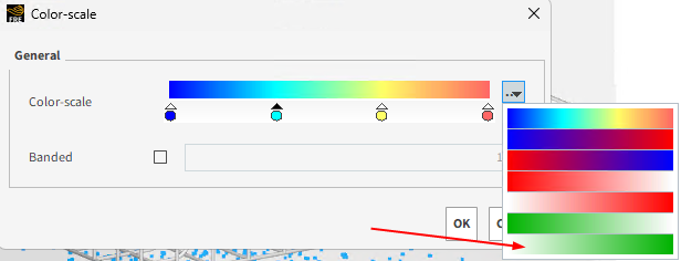
From the Color-scale dialog box, on the drop-down list, you can choose any other Color-scale configuration. Lets pick the white-to-green one.
By double-clicking inside each color mark, you can change its color. For this tutorial, let's make a blue scale instead of green.
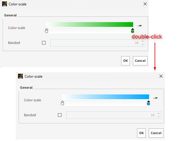
By double-clicking the center of the bar, you can add a new color mark. Double-click the center of the bar and select a light-blue (lighter than the automatically provided) for this one.
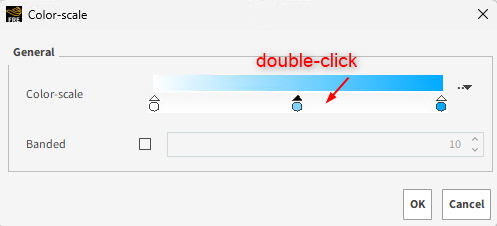
Drag this new light-blue mark to the left until it gets very close to the white one.
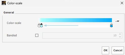
Click OK and check the new 3D View visualization.
Another topic of interest for this scenario is measuring the mass flow rates at the inlets and outlets. This measurement can be useful in the dishwasher project design to ensure that the drain releases water adequately, preventing the box from becoming full of water.
In Part A of this tutorial, we enabled the SPH Mass Flow Rate module with the inlets and drain surfaces associtaed. Now we are able to analyze these quantities.
Let's create a Time Plot to start analyzing this data.
Create a new Time Plot by clicking Ctrl + T or frolm the Windows panel by right-clicking Time Plots and selecting New Time Plot.
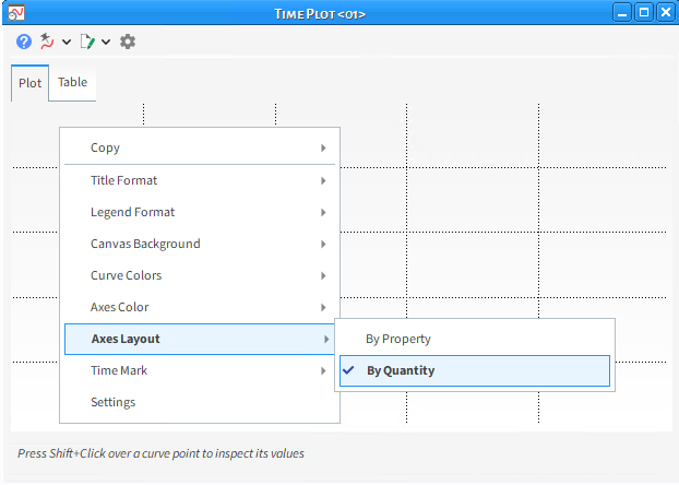
From the Time Plot background, right-click and make the Axes Layout By Quantity.
From the Data panel, multi-select the drain, inlet_01 and inlet_02 surfaces.
From the Data Editors panel, go to the Curves tab and multi-select the three Mass Flow Rate curves, as shown below.
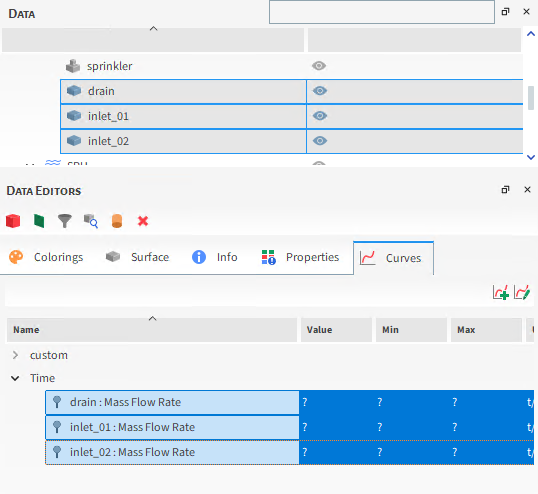
Drag and drop these curves onto the Time Plot background.
From the Data panel, select Solver, and from the Data Editors | Curves, drag and drop SPH Elements Enabled onto the plot. The resulting plot is shown below.
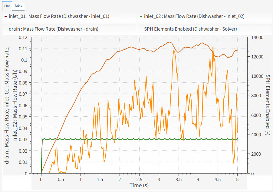
From this plot we can state that:
All three surfaces reach a steady state;
The drain releases 0.11 t/h at its peaks but releases much less most of the time, indicating that it probably has the potential to release more water than it currently does;
The dishwasher itself reaches a steady state, because the SPH Elements Enabled stabilizes, meaning that the fluid amount entering the dishwasher is roughly equal to the amount exiting.
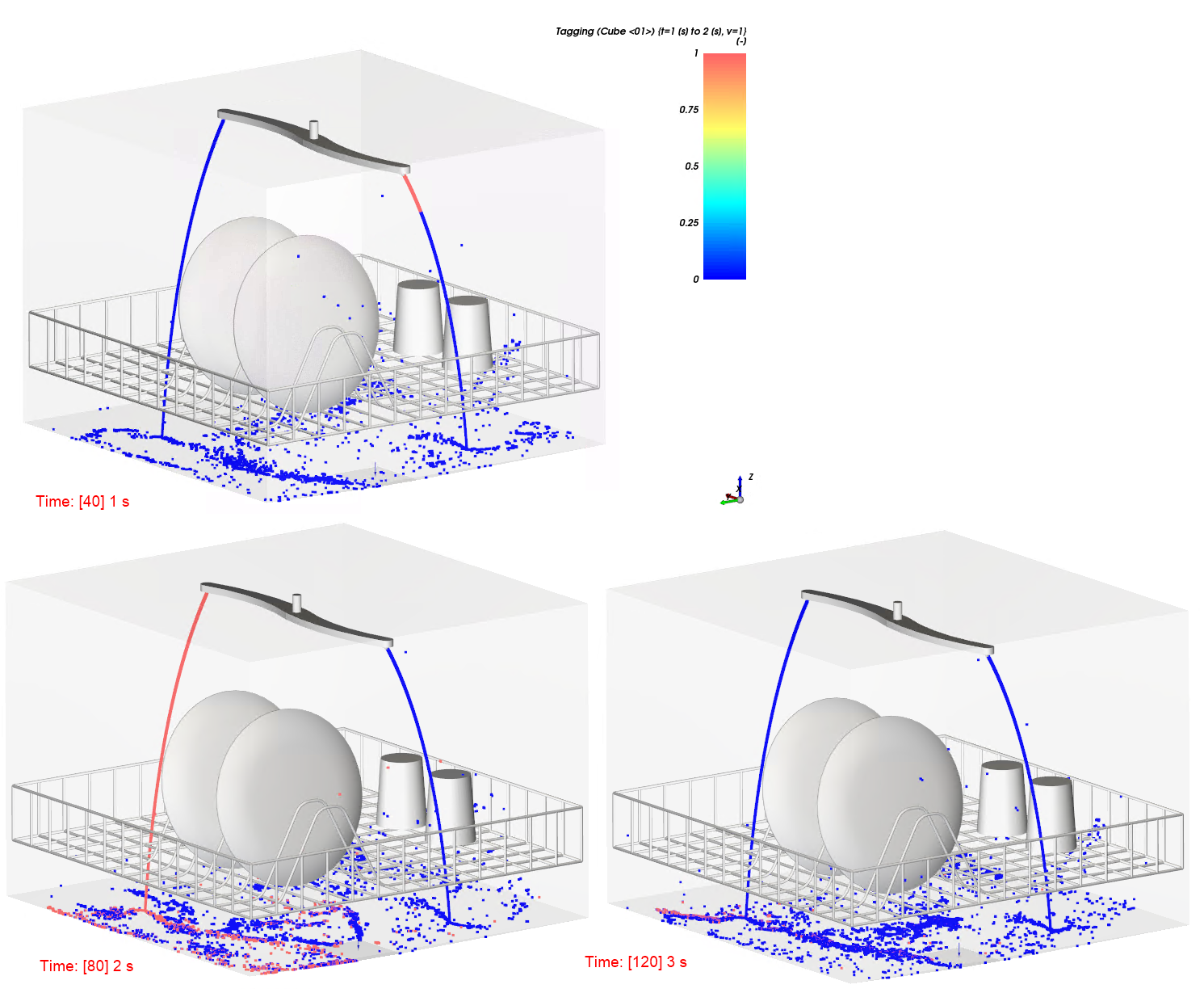
In FreeFlow, it is possible to track SPH elements by creating a Tagging Calculation.
A Tagging can be created from the main SPH entity or from User Processes created from the SPH.
Let's track, for example, the elements that were injected from inlet_02 from 1 to 2 seconds of simulation time. Follow the steps below to create this Tagging.
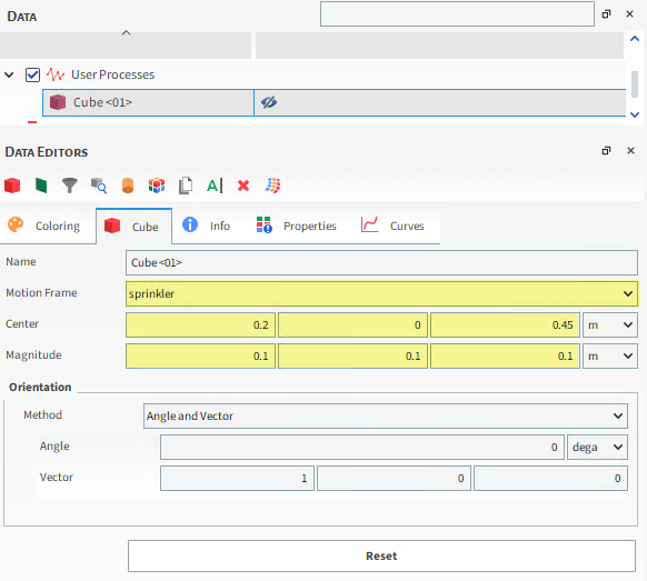
From Data panel, right-click SPH, point to Processes | Cube. A new Cube <01> is created.
From the Data Editors panel, set the Motion Frame, Center and Magnitude for the cube.
From the Data panel, right-click SPH, point to SPH Calculations | Tagging and select Cube <01>. A new Tagging (Cube <01>) entity is created under Calculations.
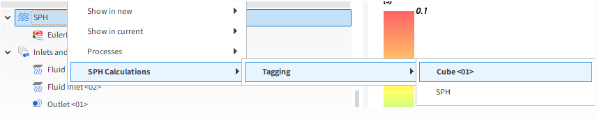
Select this new Tagging entity and from the Data Editors set the Domain Range, Initial and Final times.
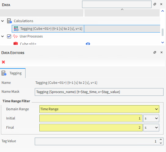
Tip: At this point, the Tagging is created and associated to a Cube that covers the inlet_02 release area and rotates together with it. This way, it will tag every SPH elements that the inlet injects between 1 and 2 seconds.
Finally, select SPH again and on the Data Editors panel, go to Coloring tab. Color the elements with the Tagging by defining Nodes | Grid-function.
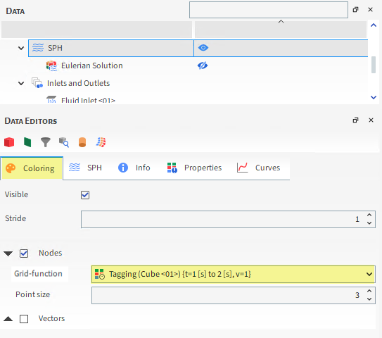
Move the time slider through different outputs to track these elements.