


The purpose of this tutorial is to run a dishwasher simulation and postprocess it in order to analyze the wet regions of the dishes, the influence of each fluid inlet on the wetting, and the drain mass flow rate.
You will learn how to:
Import Surface and Wall Geometries
Disable a Wall
Set SPH Boundary Conditions
Enable a Module
Create a Motion Frame for geometries
Create a Fluid Inlet
Create an Outlet
Process (run) the simulation
And you will use these features:
Modules
Motion Frames
Materials
Inlets and Outlets
This tutorial assumes that you are already familiar with the FreeFlow user interface (UI) and with the project workflow.
If this is not the case, please refer to Tutorial 01 - Dam Break for a basic introduction about FreeFlow usage before beginning this tutorial.
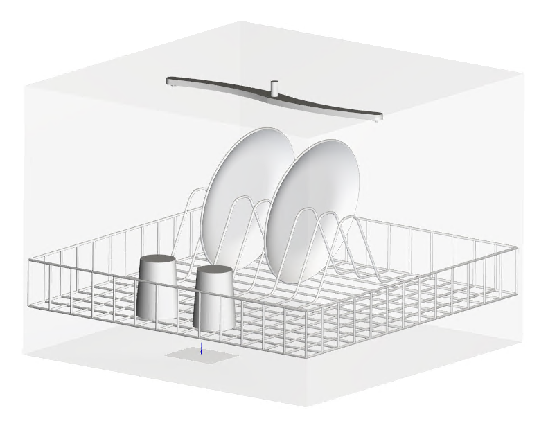
The wall geometries in this tutorial are composed of:
(1) box
(2) grids
(3) glasses
(4) plates
(5) sprinkler
In the tutorial files folder (presented below), each .stl file can be found (also for inlets and outlet surfaces).
To get started with this tutorial, do the following:
Download the
freeflow_tut02_files.zipfile here .Unzip
freeflow_tut02_files.zipto your working directory.Open FreeFlow 2026 R1.
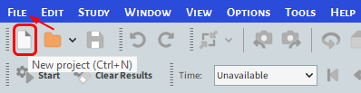
From the FreeFlow program, click the New Project button, or from the File menu, click New Project (Ctrl+N).
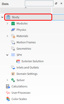
The Study entity covers the first step of the simulation setup. The purpose is to define any useful information for the project.
From the Data panel, click Study.
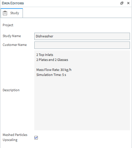
From the Data Editors panel, enter the project information.
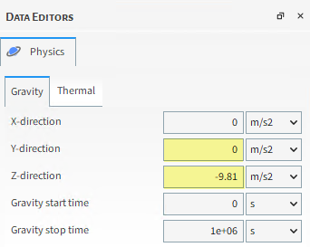
In the Physics step, we will set the Gravity in Z-direction due to the Geometries orientation for this project.
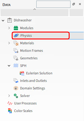
From the Data panel, click Physics.
From the Data Editors panel, set Gravity for Y and Z-directions.
For this case we will import geometry files in .stl format for both the walls and surfaces (to associate with the inlets and outlet of the simulation). To import the wall components, follow the steps below.
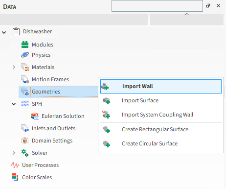
From the Data panel, right-click Geometries, and then click Import Wall.
From the Select file to import dialog, navigate to the tutorial_02_input_files folder that you previously downloaded, find the geometry folder, and then while pressing either the Ctrl or Shift key, multi-select all of the following files:
box.stl
glass_01.stl
glass_02.stl
grids.stl
plate_01.stl
plate_02.stl
sprinkler.stl
Click Open.
If you haven't saved your project yet, a Save File dialog will appear. Select a folder location, enter a File name, and then click Save.
After saving the project, a FreeFlow dialog is displayed, where geometry limits (in X, Y and Z directions) are shown.
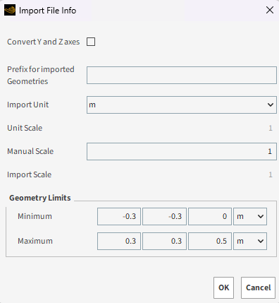
Import Unit defines the unit with which the geometry was saved previously.
For this tutorial, all geometries are in "m" (default option).
Review that the Geometry Limits match with the image.
Click OK to add the new parts into the simulation project.
Now let's import the surfaces that we will later define as inlets and outlet for the fluid.
From the Data panel, right-click Geometries, and then click Import Surface.
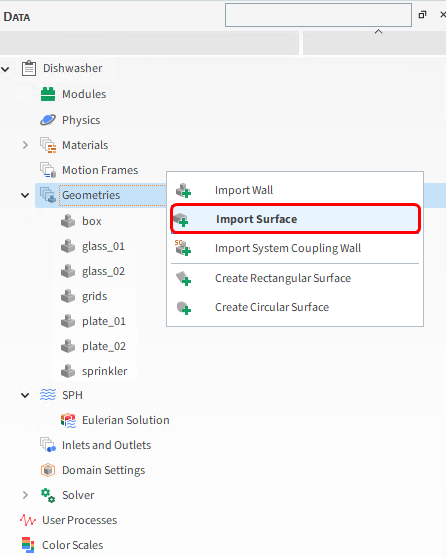
From the Select file to import dialog, navigate to the tutorial_02_input_files folder that you previously downloaded, find the geometry folder, and then while pressing either the Ctrl or Shift key, multi-select all of the following files:
drain.stl
inlet_01.stl
inlet_02.stl
Click Open.
Review the Geometry Limits.
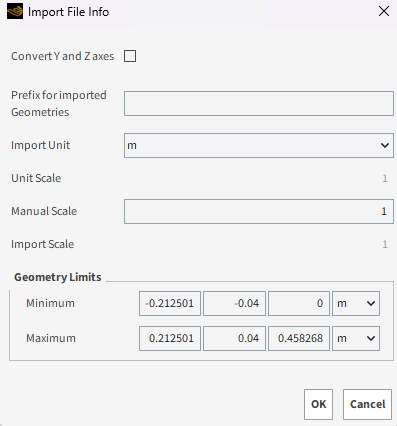
Click OK to add the new parts into the simulation project.
Tip: .stl files are not saved with an embedded unit so ensure you select the correct unit during geometry import.
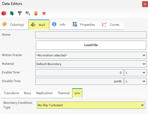
Let's define SPH Boundary Condition for the walls as No Slip Turbulent.
From the Data panel, multi-select box, glass_01, glass_02, plate_01 and plate_02 geometries.
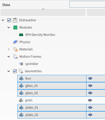
From the Data Editors panel, in the main Wall tab, select the SPH sub-tab and define the Boundary Condition Type.
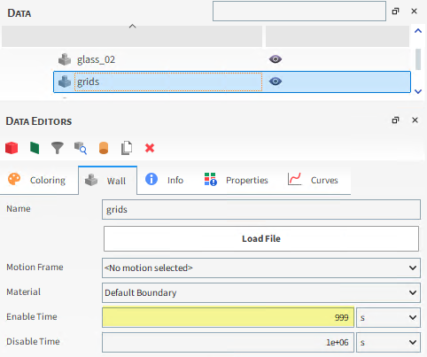
Now let's disable the grids geometry to simplify the simulation setup, so the fluid will not interact with this wall.
From the Data panel, select the grids geometry.
From the Data Editors panel, define the Enable Time.
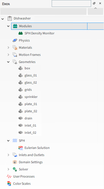
To enable the Module for this tutorial, do the following:
From the Data panel, select Modules.
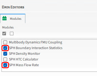
From the Data Editors panel, under Modules enable both the SPH Boundary Interaction Statistics and the SPH Mass Flow Rate checkboxes.
From the Data panel, select SPH Boundary Interaction Statistics.
From Data Editors panel, enable the Wetting Parameters checkbox.
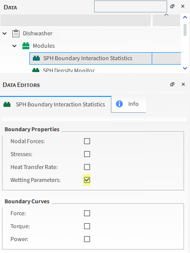
Note: By doing this, the module will collect wetting parameters for the boundaries.
The Boundary Properties field enables values for each boundary (wall) triangle for each output time, that will be useful for postprocessing analysis in this case.
From the Data panel, select SPH Mass Flow Rate.
Note: For postprocessing analysis, we want to measure the mass flow rate in the drain, so let's add it as a control surface.
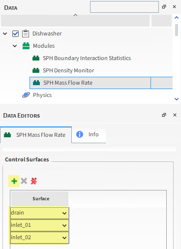
From the Data Editors panel, click Add (green plus) until you have 3 Surface rows, and select the drain, inlet_01 and inlet_02 as Control Surfaces.
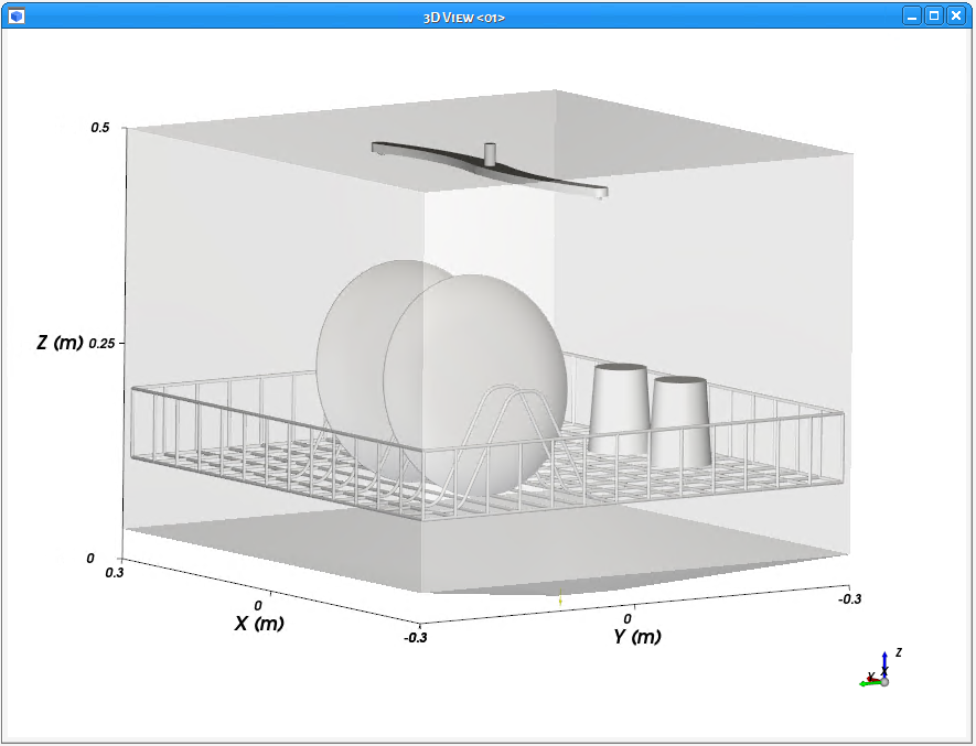
To visualize the freshly imported geometries, do the following:
From the Data panel, click and hold the Geometries entity.
Drag and drop it on top of the Workspace. The workspace will then be filled with a 3D View window of the geometries.
In this tutorial, the sprinkler and the inlets surfaces will rotate in order to distribute the fluid and wash the dishes.
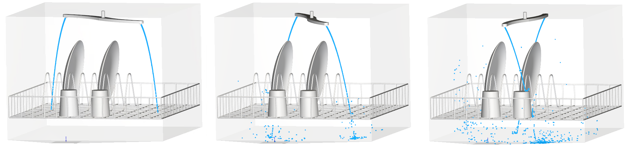
To compute the rotation movement, a motion frame of the type Rotation must to be defined and assigned to the referred geometries.
After selecting Rotation, the following options will be available:
Initial Angular Velocity: The angular velocity at the Start Time.
Angular Acceleration: The rate of change of the angular velocity.
To add a new Motion Frame, do the following:
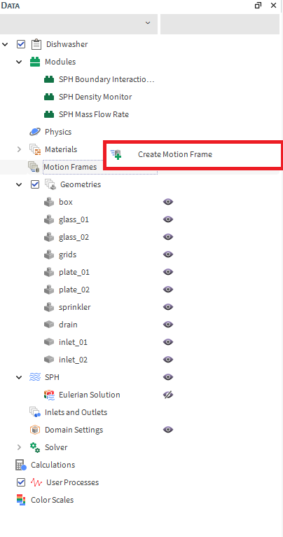
From the Data panel, right-click Motion Frames and then select Create Motion Frame.
From the Data panel, under Motion Frames, select the newly added Frame <01> entry.
From the Data Editors panel, on the Frame tab, change the Name.
From the same tab, click Add motion (green plus button), select Rotation for Type and define the Initial Angular Velocity and unit.
Tip: This way, a rotation with constant velocity around the Z axis will be defined.
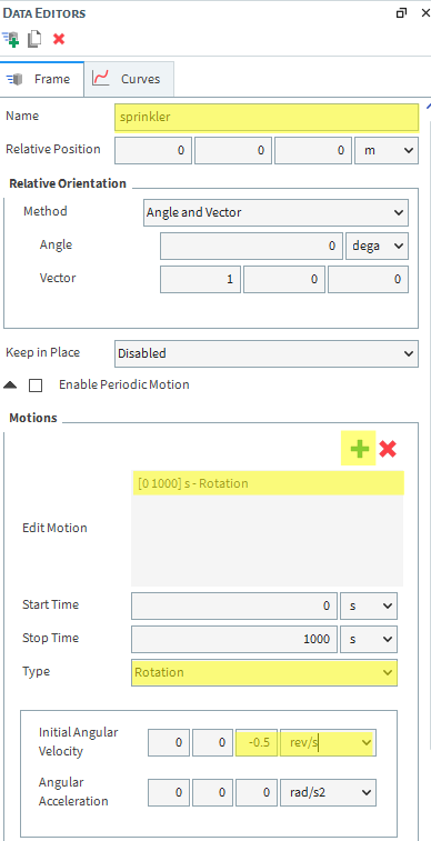
Once the Motion Frame has been created, it must be assigned to the geometries (sprinkler and inlets).
From the Data panel, under Geometries, multi-select inlet_01 and inlet_02.
From the Data Editors panel, on the Surface tab, select sprinkler from the Motion Frame drop-down list.
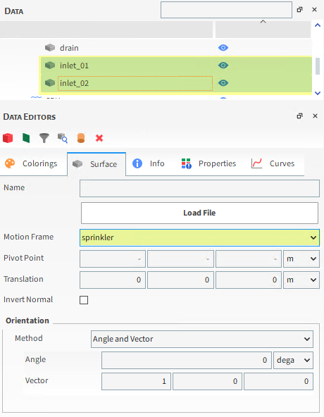
From the Data panel, under Geometries, select sprinkler.
From the Data Editors panel, on the Wall tab, select sprinkler from the Motion Frame drop-down list.
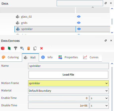
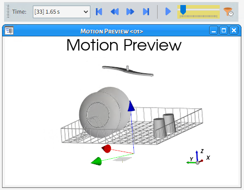
The sprinkler (and inlets) movement can be previewed using the Motion Preview window.
From the Data panel, select Motion Frames.
From the Data Editors panel, click Preview. A new window will appear showing the geometries and the created Frame.
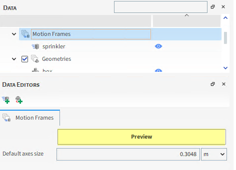
Tip: Hide the box component in order to visualize the rotating entities.
Note: The Time toolbar can be used to play the preview. The yellow color of the slider indicates that the simulation has not yet been processed.
As we want to simulate water, the default values for materials will be maintained.
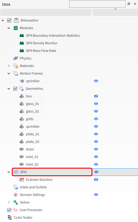
The SPH step allows you to define which Solver model (WCSPH, IISPH or DFSPH, which is a Beta solver) you will use, and also fluid dynamics, kernel, positions correction and advanced SPH parameters.
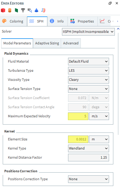
For this tutorial, default values for every parameter but for Element Size and Sound Speed will be used. These last two will be set in order to have consistent results and reduce simulation time.
Note: We are using the IISPH Solver for this tutorial.
From the Data panel, select the SPH entity, and from the Data Editors, on the Model Parameters tab, define the Maximum Expected Velocity and Element Size.
Tip: Check the SPH Technical Manual for more information on these parameters (access it through FreeFlow menu | Help | Ansys Rocky Resources).
Set your preference color for the fluid (SPH elements) from the Coloring tab on Node color.
For this tutorial, we will create two Fluid Inlets to inject fluid in the simulation and one Outlet to simulate the dishwasher drain.
From the Data panel, right-click Inlets and Outlets and then click Create Fluid Inlet.
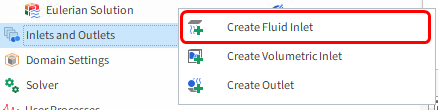
With this, a new Fluid Inlet <01> entity appears.
From the Data panel, select this new entity.

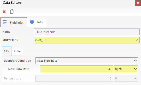
From the Data Editors panel, associate the inlet_01 as the Entry Point.
From the SPH sub-tab, define the Mass Flow Rate and unit.
 h
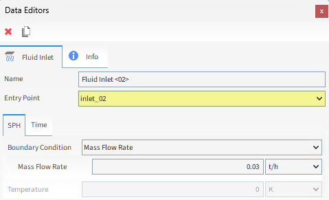
hFrom the Data panel, right-click the Fluid Inlet <01> and select Duplicate. A new Fluid Inlet <02> is created.
From the Data panel, select the Fluid Inlet <02> and from the Data Editors panel define the inlet_02 as the Entry Point for this one.
Now let's create the outlet and associate it with the drain surface.
From the Data panel, right-click Inlets and Outletsand then click Create Outlet.
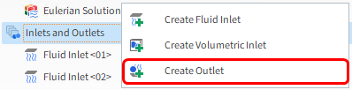
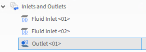
With this, a new Outlet <01> appears.
From the Data panel, select this new entity.
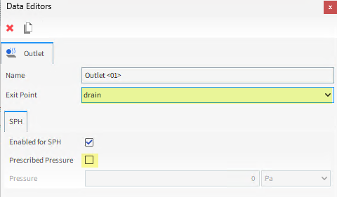
From the Data Editors panel, associate the drain as the Exit Point and disable the Prescribed Pressure checkbox.
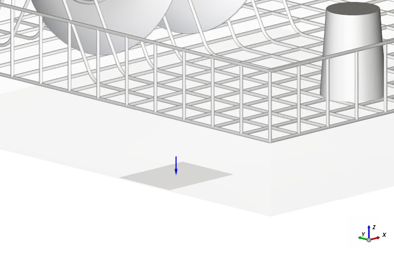
You can see the created Outlet in the 3D View with an arrow indicating the flow direction.
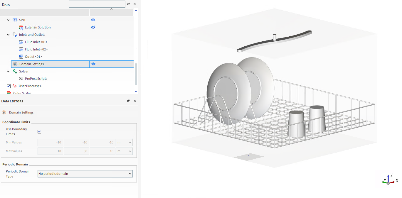
For the Domain Settings step, we will use the boundary limits (let the Boundary Limits checkbox marked as it is by default).
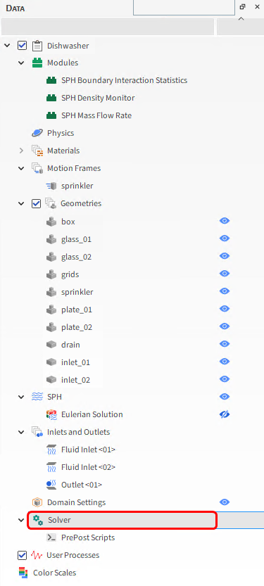
The Solver step is where you define processing time and stability details, and finally Start processing your simulation.
Follow the steps below to set up the solver:
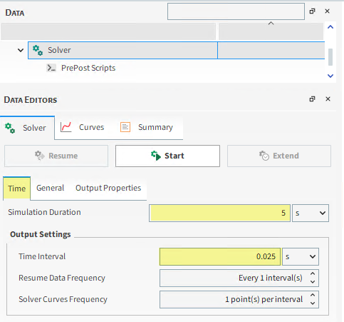
From the Data panel, click Solver, and then from the Data Editors panel, select the Solver | Time tab. Define Simulation Duration and Output Settings | Time Interval.
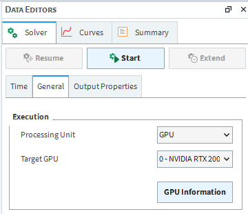
From the General sub-tab, select what you want for Processing Unit, and then the Target GPU(s) (or Number of Processors). For this tutorial, GPU will be faster.
Click the Start button to begin processing.
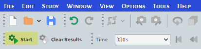
Note: After defining Solver options, it is also possible to begin processing using the Start button from the Simulation Toolbar.
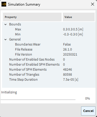
Once you click Start, the Simulation Summary window will appear. It shows the geometry bounds, number of triangles, and the calculated Timestep Duration.
This window will disappear on its own, then processing begins.
This completes Part A of this tutorial.
For further information on any topic presented, we suggest searching the User Manual, which provides in-depth descriptions of the tools and parameters.
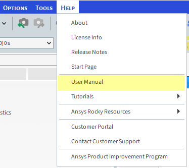
To access this manual, from the main Toolbar click Help and then click User Manual.
FreeFlow was used to set up and process a dishwasher simulation.
During this tutorial, it was possible to:
Enable a Module
Import Walls and Surfaces
Disable a Wall
Set SPH Boundary Conditions
Define Fluid and Fluid Inlet
Define an Outlet
What's Next?
If you completed this tutorial successfully, then you are ready to move on to Part B and post-process this project.