Introduce some basic methods for analyzing a simulation after it has been processed.
The purpose of this tutorial is to introduce some basic methods for analyzing a simulation after you have processed it. We will continue from where we left off in Part A.
You will learn how to:
Create an Animation
Visualize Properties in a 3D View Window
Create Graphs and Plots
Filter data with User Processes
Export results
And you will use these features:
Animation panel (videos)
Time toolbar
Multi Time plot
Time plot
Cube User Process
Plane User Process
If you completed Part A of this tutorial, ensure that FreeFlow project is open (Part B will continue from where Part A left off).
Download the
freeflow_tut01_files.zipfile here .Unzip
freeflow_tut01_files.zipto your working directory.Open FreeFlow 2026 R1.
Important: To make use of the FreeFlow project file provided, you must have FreeFlow 2026 R1 or later. If you have an earlier version of FreeFlow, please upgrade to the latest version, or complete Part A from scratch.
From the FreeFlow program, click the Open Project button, find the
freeflow_tut01_filesfolder, and then from thetutorial_01_A_pre-processingfolder, open thetutorial_01_pre-processing.freeflowfile.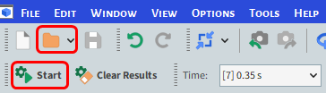
Process the simulation. (From the Simulation toolbar, click the Start button.)
Now that the project has completed processing, we can begin to analyze it. For example, you can use the Time toolbar in the following ways:
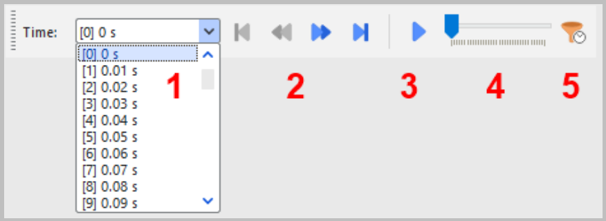
Select a specific output/time from the drop-down list
Use the arrow buttons (from left-to-right) to:
Go to first output
Step back one output
Step forward one output
Go to last output
Play the simulation animation
Slide to the output you want using the slider bar
Use the Timeset Filter to display only a specified time range
There are 3 different ways to color the boundaries and/or the elements:
Use the Coloring toolbar to color all the boundaries/SPH elements by a property.

Use the Properties tab from the Data Editors by dragging and dropping the desired property over a 3D View window.
Use the Coloring tab by doing the following:
From the Data panel, select either a wall under Geometries or the main SPH entity.
From the Data Editors panel, select the Coloring tab and then select the desired property to color (for the Wall, Faces, Edges and Nodes or for the SPH, Nodes and Vectors).
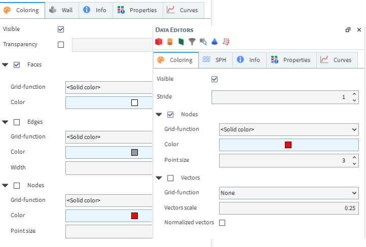
For this tutorial, we want to color our fluid elements by velocity.
From the Data panel, select SPH and then from the Data Editors panel, select the Properties tab.
Select Velocity and then drag and drop it onto the 3D View window.
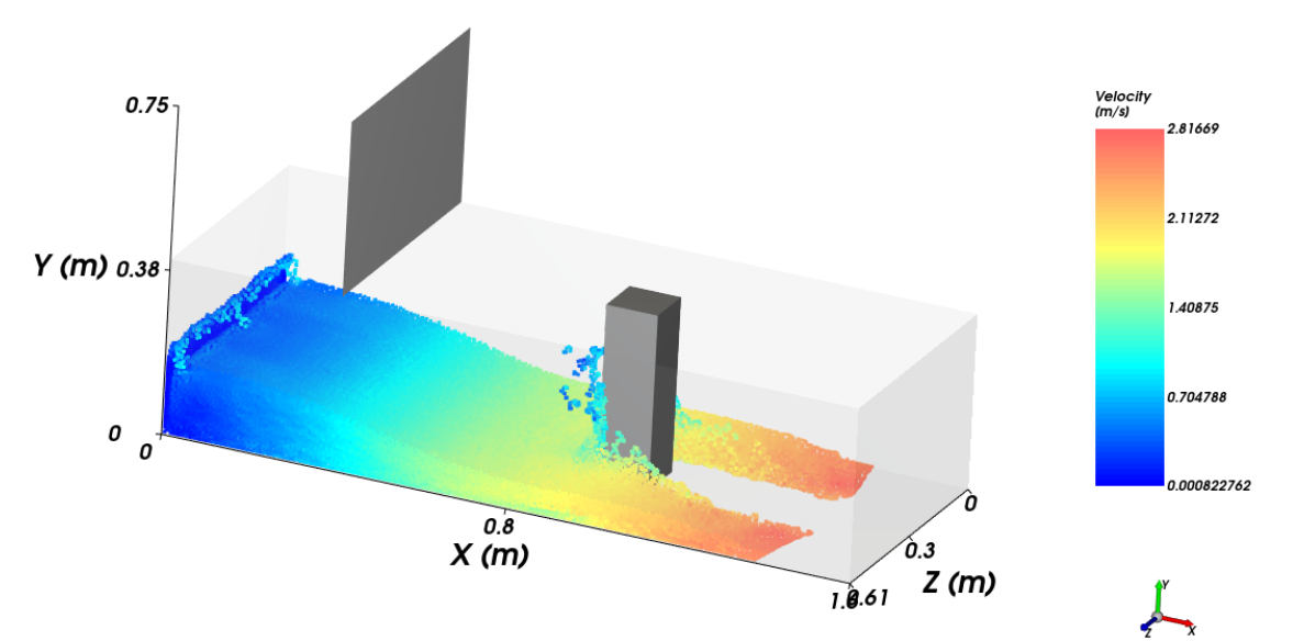
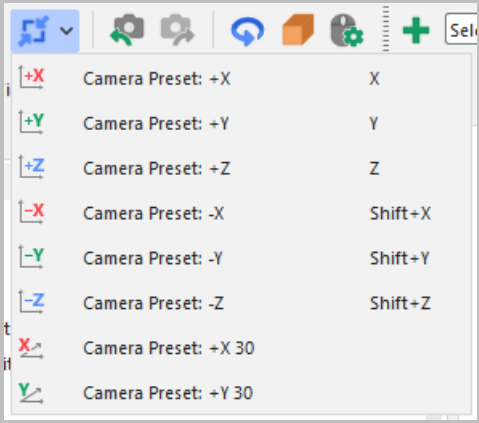
You can then use your mouse to zoom and pan, and use your mouse or the options on the Fit toolbar (as shown) to change the orientation.
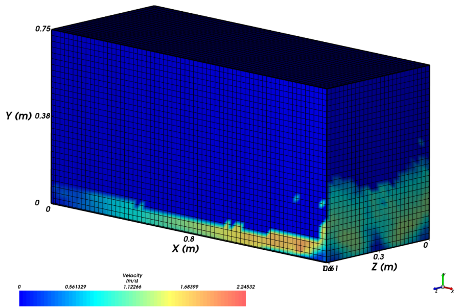
To represent SPH data as continuous fluid, we will use the Eulerian Solution to continue the postprocessing.
We will first color the cells by Velocity, in order to compare the results we had by coloring the SPH elements.
From the Data panel, on the SPH field, select Eulerian Solution and then from the Data Editors panel, select the Coloring tab.
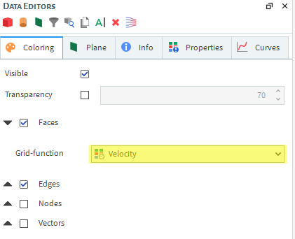
Expand Faces and then select Velocity from the drop down list as Grid-function.
Use the eye icons to make Eulerian Solution visible and hide everything else but the Velocity color scale.
Note: You will view only data from the most external cells from the domain. To see results from an specific area, you can create a cube, cylinder or a plane User Process from the Eulerian Solution entity and follow the same procedure.
For some SPH analyses the data must be restricted to a particular region, or a particular subset of fluid.
FreeFlow User Processes are used to divide and analyze SPH elements, Eulerian Solution and wall Geometries, and include the following types:
Cube: Create a subset of data based upon a box region.
Cylinder: Create a subset of data based upon a cylinder region.
Plane: Create a subset of data based upon a plane.
Filter: Create a subset of fluid/geometry based upon a particular property value or range.
Cell Inspector: Select a single, individual fluid element or triangle (boundary).
Eulerian Statistics: Transform the discrete properties into continuous values by averaging the values over discretized regions.
Note: Eulerian Statistics can only be created from a SPH Cube or Cylinder.
PLANE
In this tutorial, we are interested in analyzing the region where Water collides with the column.
Let’s create a Plane in order to visualize the middle of the container and continue analyzing the fluid velocity with the Eulerian Solution.
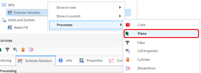
From the Data panel, right-click Eulerian Solution, select Processes and then Plane.
From the Data Editors panel, define Orientation Angle and Vector.
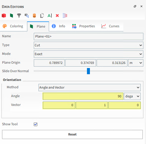
Navigate to the Coloring tab, uncheck Edges, ensure Faces is enabled, expand it and then select Velocity from the drop-down list as Grid-function.
CUBE
We will also restrict the middle of the domain with a Cube for the elements to compare the SPH with the Eulerian Solution view .
In order to make the comparison between the views, create a new 3D View by using the shortcut Ctrl+D.
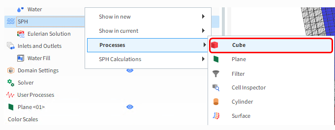
From the Data panel, right-click SPH, select Processes and then Cube.
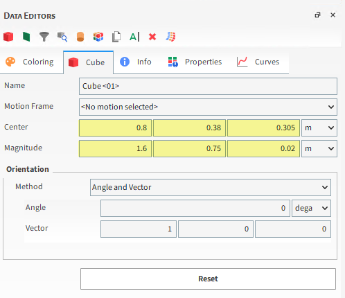
From the Data Editors panel, define Center and Magnitude.
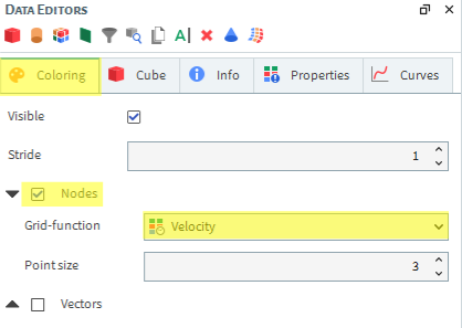
Navigate to the Coloring tab, ensure that the Nodes field is enabled, and then select Velocity from the drop-down list as Grid-function.
USER PROCESSES IN DATA PANEL
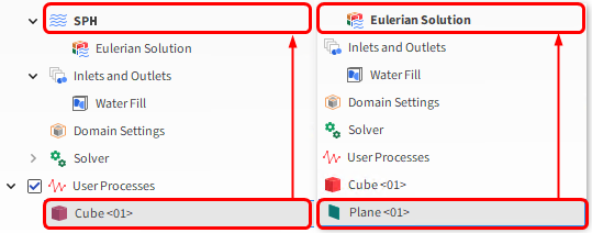
When a User Process is selected in the Data panel, FreeFlow highlights the association between it and other User Processes by displaying the parent User Process name in bold.
So, when you select Cube <01>, SPH will be displayed in bold letters, and when you select Plane <01>, the same happens with Eulerian Solution. Take a moment to check it from your project.
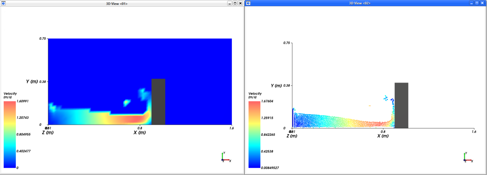
Finally, let’s visualize and compare the fluid views between SPH (discrete) and Eulerian Solution (continuous) data.
From the Windows panel, select the 3D View <01> and use the eye icons to hide everything but the Plane <01>, column and Velocity color scale.
Select the 3D View <02> and use the eye icons to hide everything but the Cube <01>, column and Velocity color scale.
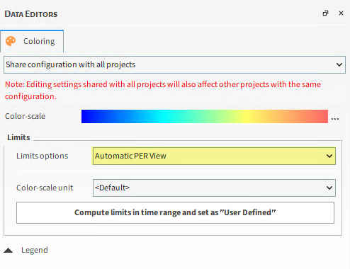
On the Data panel, from Color Scales, select Velocity, and from the Data Editors panel, ensure Limits options is defined as Automatic PER View.
Use the mouse to adjust the views in a way you can compare them.
Tip: If you are using a full screen in the workspace, use the button located on the upper right in order to make the window adjustable.
Use the slider from the time bar to choose the timestep you want to analyze.
We will also make use of a Filter User Process in order to visualize a fluid surface.
WEIGHT GRID-FUNCTION
To represent it, we will restrict Eulerian Solution data based upon a value for a grid-function defined as Weight.
The value of the properties (velocity, density, etc.) for each node of the interpolation grid is based on an interpolation, using the kernel function, of the values of the SPH elements inside the kernel radius.
Tip: Refer to FreeFlow Technical Manual to learn more about Kernel functions.
The Weight grid-function gives the summation of the weight of all SPH elements that affect each grid node.
This property can be used to define the fluid surface as it gives the density of SPH elements around the nodes.
If the region has no SPH elements, the Weight returns 0.
When the region is full of elements, the function tends to return a value close to 1.
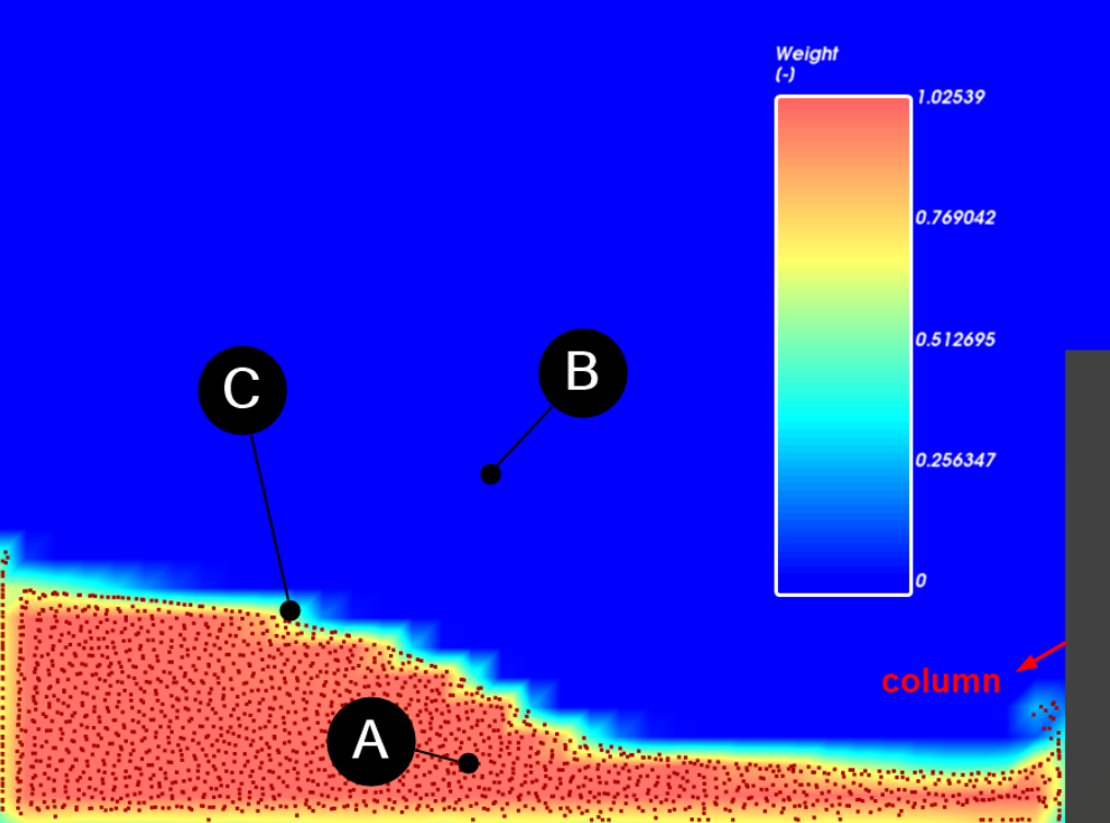
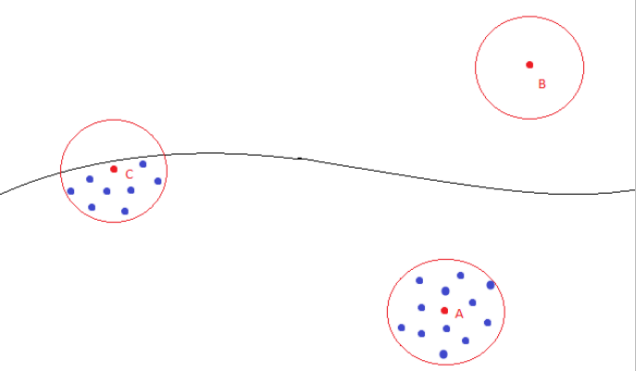
To better understand how the Weight is calculated, see the images below.
Point A: ≈ 1
Point B: 0
Point C: 0 < Weight < 1
As the volume around C is half empty, half full of elements, Weight tends to return ≈ 0.5 (see the Color Scale).
WATER SURFACE VIEW
To visualize the desired fluid surface, let’s create a weight based isosurface.
From the Data panel, right-click Eulerian Solution, point to Processes and then Filter.
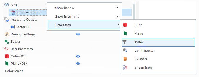
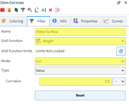
Select Filter <01> and from the Data Editors panel, define the Name, Grid-function, Mode and Cut value.
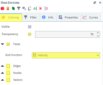
From Data Editors panel, select the Coloring tab, enable Transparency checkbox, and ensure Faces is enabled while Edges, Nodes and Vectors are disabled.
Expand Faces and select Velocity as Grid-function.
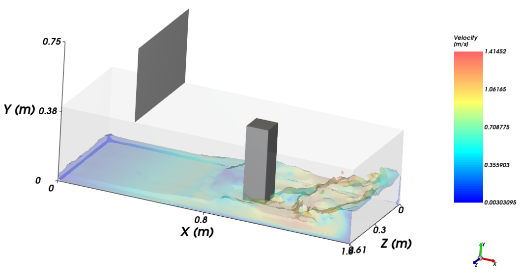
You can visualize the resulting surface for all timesteps in a 3D View.
To create an animation (video) in FreeFlow, you set key frames of a particular 3D View window at specified outputs.
FreeFlow will interpolate between the created key frames using the available outputs saved during the simulation.
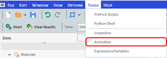
To show the Animation panel, from the Tools menu, select Animation.
ANIMATION PANEL
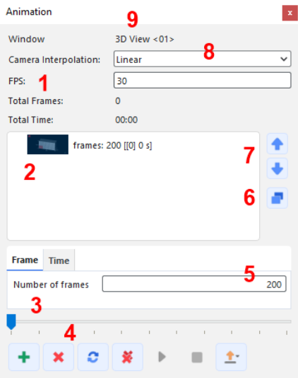
Frames per Second (FPS) will change the playback speed of the animation. At least 30 FPS is recommended. To create a smooth animation, the Time Interval should not be greater than 1/FPS.
Key Frames list.
Select a specific moment in the animation.
Add Key Frame / Remove Key Frame / Update Current Key Frame / Remove All Key Frames / Play / Stop / Export (video or images).
Number of frames between the selected Key Frame and the next one. The Number of Frames divided by the FPS gives the real animation time. This value can be changed to display the animation in real time.
Duplicate the selected Key Frame.
Move the selected Key Frame Up or Down to change the order.
Camera Interpolation method.
Name of 3D View window that is currently selected.
For this tutorial, a simple animation using only 2 Key Frames in real time will be created (3.5 s).
Since we use an Time Interval of 0.01 s, we should use an FPS of 100 or less (FPS should be less than or equal to 1/Time Interval). Use FPS 100 (as shown).
Select the 3D View you set up to visualize the water surface. Then, using the Time toolbar, change the output to 0 s.
Add the first Key Frame by clicking the Add Key Frame (green plus) button.
Select the new frame and then from the Frame tab, change the Number of Frames to 350 (as shown). Since there are 350 output files in this simulation, and our FPS is 100, this will give us the full 3.5 seconds between our first and second frames (350 / 100 = 3.5).
Use the Time toolbar to change the time to the last output, and add a second Key Frame.
Your Total Time should be 00:03 (real time).
Click Play to preview the movie in the 3D View window.
Click Export Animation to save the movie to an .avi file.
All the Properties are calculated for every timestep and every Triangle (wall mesh) or Fluid element (SPH).
In order to create a Time Plot or a Multi Time Plot, you must select one of the following operations to transform the Properties into a single time-dependent curve:
Minimum: Lowest value among all elements/triangles
Maximum: Highest value among all elements/triangles
Sum: Sum of all values among all elements/triangles
Sum Squared: Sum of the squared values among all elements/triangles
Average: Mean value among all elements/triangles
Variance: Squared deviation of a value from its mean
Standard Deviation: Squared root of the variance
The Solver entity contains a Curves tab, which includes several pre-defined curves that can be plotted without applying any additional operations.
Because we enabled the SPH Boundary Interaction Statistics module, for this tutorial, every Wall also contains a Curves tab.
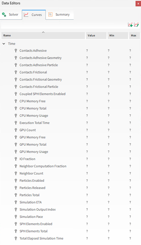
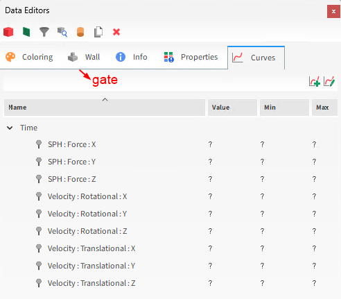
Note: Entities with Motion Frames will also have a Curves tab with motion data. This way, the gate will have curves for both motion and interactions data.
TIME PLOT
The Time Plot is a useful tool to analyze a single curve, or to compare different curves at the same time, plotted on the same grid.
In this tutorial we will analyze the resulting fluid force in the column in the X (fluid flow) direction for all timesteps.
We will also visualize the maximum fluid force in a column triangle in order to see where it occurs in the wall.
To create a Time Plot, do the following:
From the Windows panel select New Time Plot, or use the shortcut Ctrl+T.
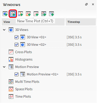
From the Data panel, select column and then from the Data Editors panel, select the Curves tab.
From the Curves tab, drag and drop SPH : Force : X over the time plot window.
From the Properties tab, right-click SPH : Force : Nodal : X, point to Time Plot, then Show in selected Time Plot, and click in Max.
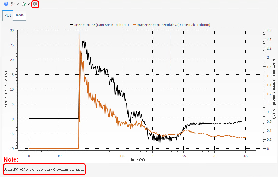
Note: You can inspect the plotted values by pressing Shift+Click over a curve.
In the top left corner of the plot, you can select Configure Window to edit text display, colors, axes limits, units and other related options.
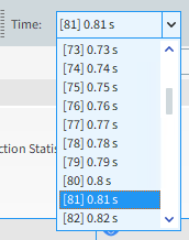
By inspecting the values, it is possible to see that the maximum force value in a column triangle occurs at 0.81 s.
Note: Your results may differ slightly from the ones presented in this tutorial.
Let’s color the column in a 3D View by nodal forces to see the point of the wall (the triangle) that the force is occurring.
Select or create a 3D View and follow the steps below.
From the Data panel, select column.
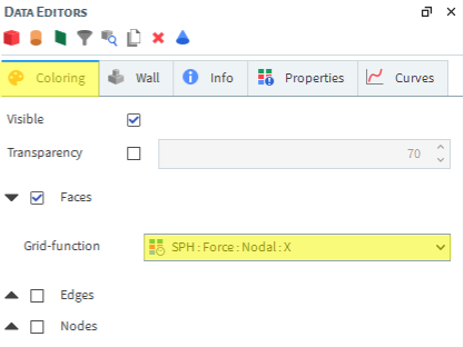
From the Data Editors panel, go to the Coloring tab, ensure Faces is enabled and select SPH : Force : Nodal : X as Grid-function.
From the Time Toolbar, select the time that the maximum force occurs (in this tutorial, 0.81 s).
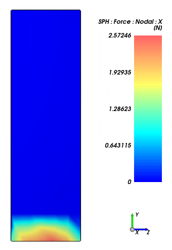
You can visualize the point where the maximum fluid force occurs in the 3D View by hiding everything but the column and the SPH : Force : Nodal : X Color Scale.
Note: The maximum force occurs when the water first collides with the column, in the base of the column. You can use the shortcut Shift+X to see the face in a normal view.
This completes Part B of this tutorial.
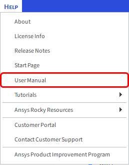
For further information on any topic presented, we suggest searching the User Manual, which provides in-depth descriptions of the tools and parameters.
To access this manual, from the main Toolbar click Help, point to Manuals, and then click User Manual.