


The purpose of this tutorial is to introduce the FreeFlow user interface, go over the various parameters, and outline the basic steps for setting up a FreeFlow project.
The scenario considered is a dam break.
You will learn how to:
Import Wall Geometries
Enable a Module
Create a Motion Frame for a wall
Configure a Fluid Material
Create an Inlet
Define a Domain
Process (run) the simulation
And you will use these features:
Modules
Motion Frames
Materials
Inlets and Outlets
Domain Settings
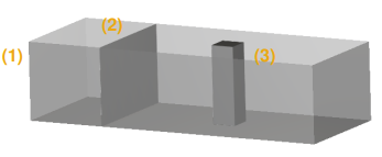
The wall geometries in this tutorial are composed of:
(1) container
(2) gate
(3) column
In the tutorial files folder (presented below), each .stl file can be found.
To get started with this tutorial, do the following:
Download the
freeflow_tut01_files.zipfile here .Unzip
freeflow_tut01_files.zipto your working directory.Open FreeFlow 2026 R1.
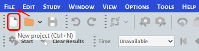
From the FreeFlow program, click the New Project button, or from the File menu, click New Project (Ctrl+N).
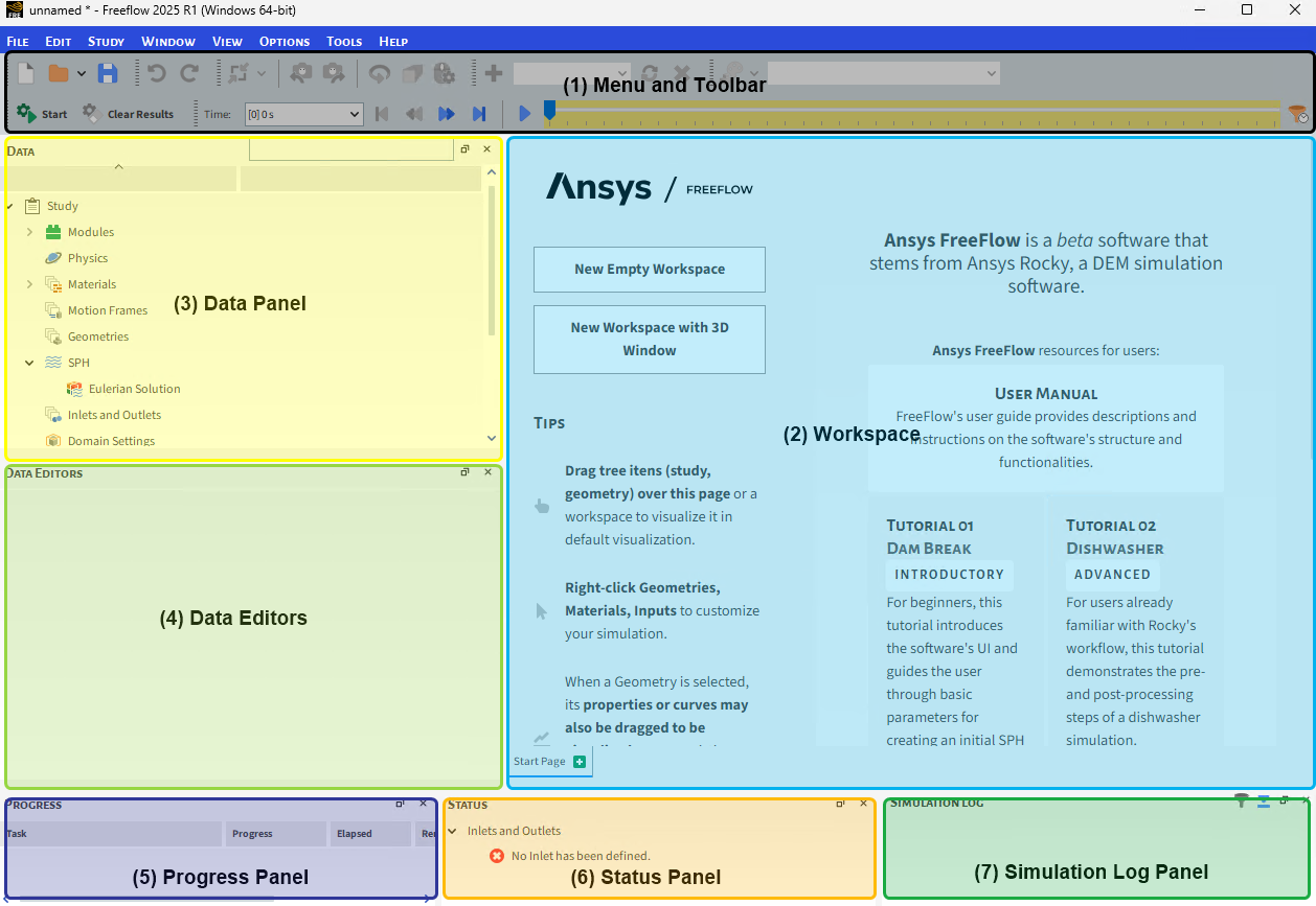
The FreeFlow user interface (UI) is customizable, you can add/remove/reposition any window or panel available. To change back to the default, select View from the main Toolbar, and then click Reset layout.
The default layout contains the following components:
(1) Menu and Toolbar: Contains the main program menus, shortcuts, camera options, time step controls, and display tools.
(2) Workspace: Displays the available windows that have been opened for the project (3D Views, Motion Previews, Plots and Histograms).
(3) Data Panel: Displays the project tree through which the setup parameters are defined.
(4) Data Editors Panel: Displays the details of the item that is selected in the Data panel.
(5) Progress Panel: Shows the processing tasks currently being performed.
(6) Status Panel: Shows any warnings or errors regarding the current project.
(7) Simulation Log Panel: Lists any Solver warnings or errors.
To set up any FreeFlow simulation, from the Data panel under Study, follow the items listed top-down and one-by-one:
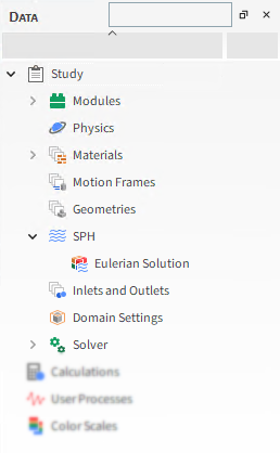
Study: Change the study name from the default (Study) and add a description.
Study also enables the activation of two other entities (for certain external Modules only) that are hidden by default:
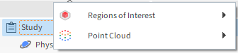
Regions of Interest: Create a Cube or Cylinder region where custom calculations can be performed.
Point Clouds: Import field data that is defined in a text file.
Modules: Enable additional models and data collection options.
Physics: Set physical conditions (Gravity and Thermal).
Materials: Define and set properties for solid and fluid materials.
Motion Frames: Add and preview movement to the simulation components (Geometries).
Geometries: Import, add, and edit geometry components.
SPH: Define SPH Solver (WCSPH, IISPH or DFSPH) and model parameters, such as fluid dynamics and kernel.
Inlets and Outlets: Define fluid inlets and/or outlets rates and release locations.
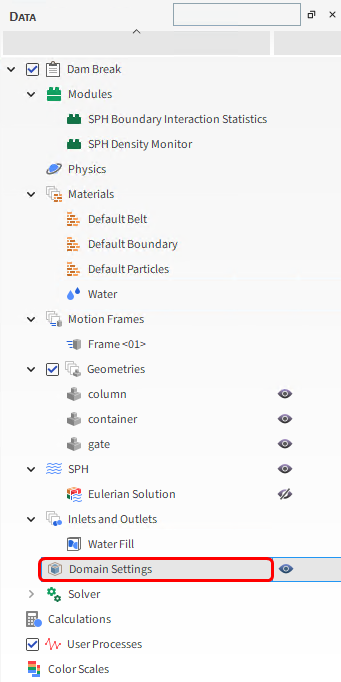
Domain Settings: Define the simulation domain coordinates and behavior.
Solver: Define how the SPH solver processes the simulation and collects data.
The remaining items at the bottom of the Data panel are for post-processing:
Calculations: Displays user-defined SPH properties, such as SPH tagging.
User Processes: Displays user-defined processes, such as analysis cubes and planes.
Color Scales: Shows display details of all plotted properties.
Note: The postprocessing is covered in Part B of this tutorial.
The Study entity covers the first step of the simulation setup. The purpose is to define any useful information for the project.
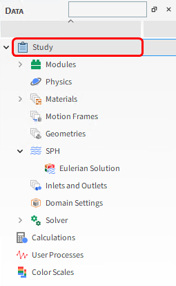
1. From the Data panel, click Study.
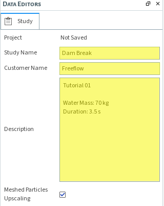
2. From the Data Editors panel, enter the project information (as shown).
In the Physics step, you can use the Gravity and Thermal tabs to configure and enable/disable these conditions.
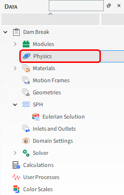
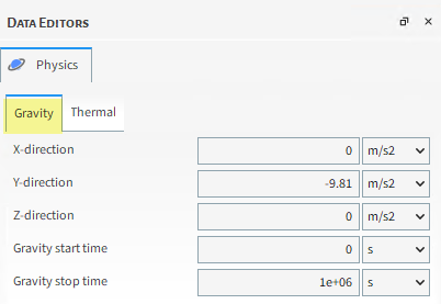
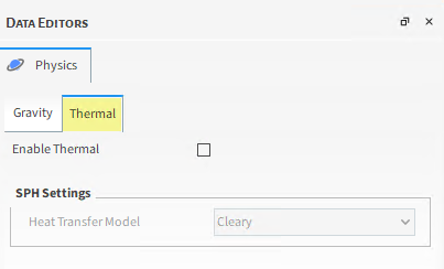
For this tutorial, we will keep all the values and settings as default.
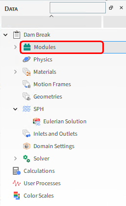
For the Modules step, we will be turning on the collection of some additional data by enabling a module.
Before taking any steps, let's understand Modules:
In FreeFlow, Modules refer to separate pieces of code that add in discrete features or functionalities within your project.
By having most of these Modules disabled by default, calculations that you may not require are avoided, which saves processing time and reduces file size.
But it also means that if you want to make use of a Module, you must remember to turn it on during your simulation setup.
In addition, some Modules add new options within other parts of the FreeFlow setup so it is important that you turn on your Modules before setting up the rest of your project.
It is also important to understand that some Module settings will override similar default settings in the FreeFlow UI.
Tip: To find out what models or settings are affected by a Module, you can view the Affected Simulation Entities information on the Module's Info tab.
There are several Modules provided by default in FreeFlow (listed below).
You may also have access to other custom Modules that are not included with FreeFlow by default.
Custom Modules are installed via .zip file from the Ready-to-use Modules page.
After installation, they will appear in FreeFlow on the Data Editors panel for Modules.
Tip: You can make your own custom Modules by using the Solver SDK functionality (see the Ansys Rocky Solver SDK Manual and the Rocky Tutorial 23 for details).
When working with Modules, it is important to realize that:
Default Modules are defined in the User and Technical Manuals, which can be found from the FreeFlow Help | Manuals menu.
Custom Modules have their own documentation that (if provided) can be launched from the Module itself.
The following Modules are available by default in FreeFlow:
SPH Boundary Interaction Statistics: Enables the collection of boundary-related collision data, such as Forces, Torque and Power.
Note: We will enable this module within this tutorial.
SPH Density Monitor: Monitors the density values associated to the SPH elements during a simulation and issues a warning if detects deviations that exceed the maximum allowed values, indicating the percentage of SPH elements that had density values clipped.
SPH HTC Calculator: Estimates the heat transfer coefficient associated to geometry triangles, based on correlations dependent on the Prandtl number and the local Reynolds number.
SPH Mass Flow Rate: Allows to add Control Surfaces to measure their liquid mass flow rate.
To enable the Module for this tutorial, do the following:
From the Data panel, select Modules.
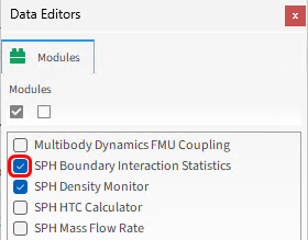
From the Data Editors panel, under Modules enable the SPH Boundary Interaction Statistics checkbox.
From the Data panel, select SPH Boundary Interaction Statistics.
From Data Editors panel, enable the Nodal Forces and Force checkboxes.
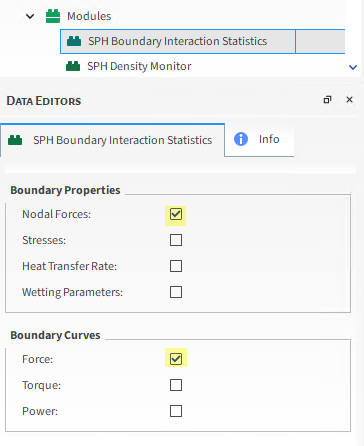
Note: By doing this, the module will collect force interaction data for the boundaries.
The Boundary Properties field enables values for each boundary (wall) triangle for each timestep, that you can make operations with.
The Boundary Curves field enables average values that correspond to the referred boundary for each timestep.
The Geometries step enables you to create (Rectangle and Circle) or import (Custom) 2D geometries that you can use as Inlets and Outlets or in postprocessing, or to import Wall geometries.
Note: A Wall is a geometry that interacts with the fluid elements.
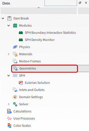
For this case we will import geometry files in .stl format.
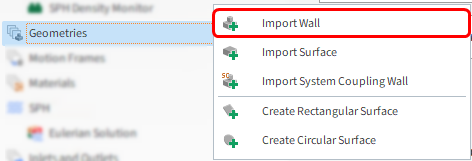
1. From the Data panel, right-click Geometries, and then click Import Wall.
The following geometry formats can be imported into FreeFlow:
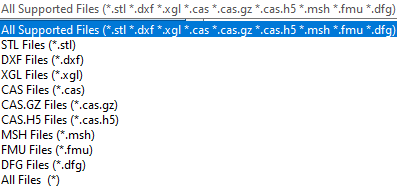
2. From the Select file to import dialog, navigate to the tutorial_01_input_files folder that you previously downloaded, find the geometry folder, and then while pressing either the Ctrl or Shift key, multi-select all of the following files:

3. Click Open.
4. If you haven't saved your project yet, a Save File dialog will appear. Select a folder location, enter a File name, and then click Save.
After saving the project, a FreeFlow dialog is displayed, where geometry limits (in X, Y and Z directions) are shown.
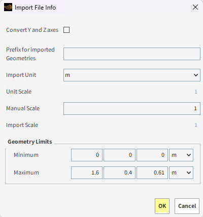
Import Unit defines the unit with which the geometry was saved previously.
5. For this tutorial, all geometries are in "m" (default option).
6. Review that the Geometry Limits match with the image.
7. Click OK to add the new parts into the simulation project.
Tip: .stl files are not saved with an embedded unit so ensure you select the correct unit during geometry import.
FreeFlow always saves your project in 2 parts:
(Project_name).freeflow: This is the Project file, which includes the simulation setup values.
(Project_name).freeflow.files: This is the Project folder, which contains all the generated configurations, logs and calculated timesteps.
To share your project, it is very important to always send both parts. FreeFlow provides an easy way to do this:
From the File menu, select Archive project. FreeFlow will create a file called (Project_name).freeflow_archive, which is a compressed file, containing both parts.
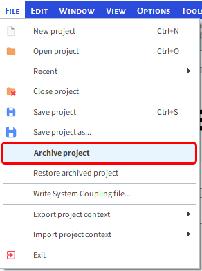
To open it, just click the File menu, and then select Restore archived project.
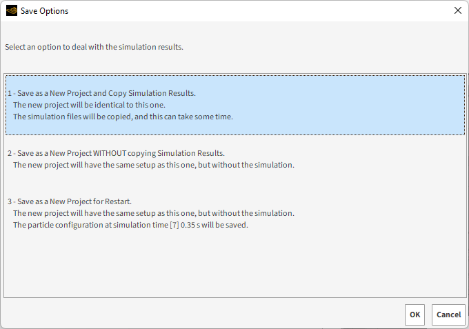
After you process your simulation, three other options for saving the project are displayed when you select Save project as. . . from the File menu, as follows:
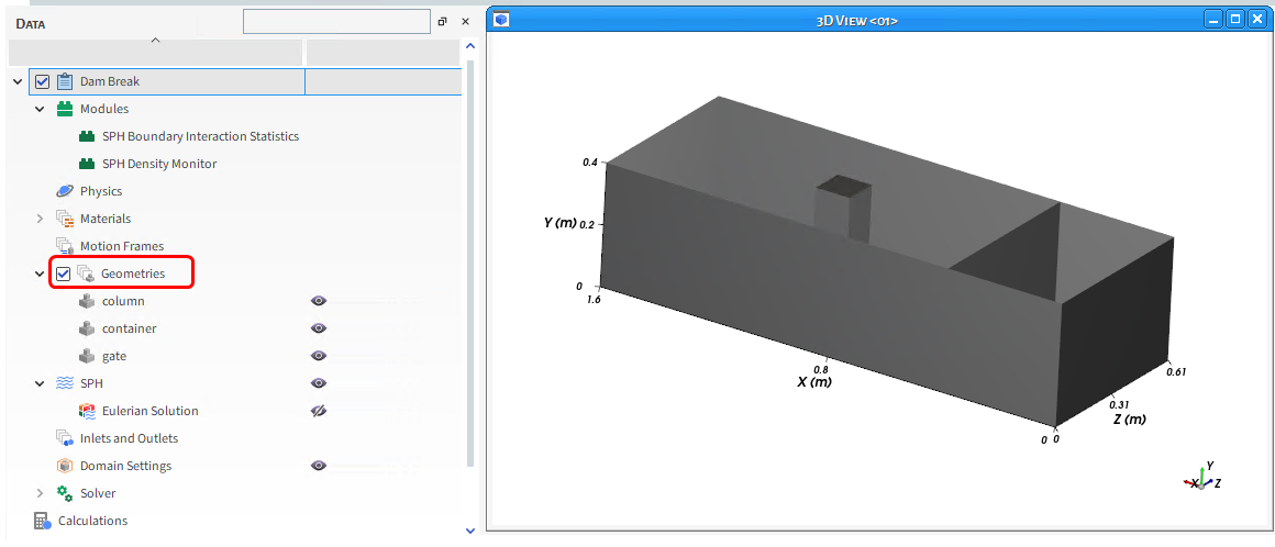
To visualize the freshly imported geometries, do the following:
From the Data panel, click and hold the Geometries entity.
Drag and drop it on top of the Workspace. The workspace will then be filled with a 3D View window of the geometries.
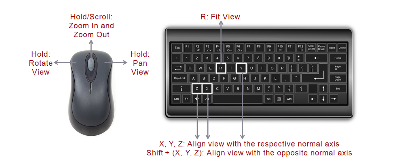
In the 3D View window, you can use the following controls and shortcuts to modify the view:
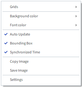
A 3D View window can be changed by right-clicking anywhere in the background (outside the geometries parts). Some configuration options include:
Grids: Allows you to change faces and edges colors for the geometries, as well as the display method.
Background and Font color: Change the color of the 3D View background and the text displayed in the window.
Auto Update: Enable/disable update of the graphical 3D View regarding any modification in the Data panel.
Bounding Box: Enable/disable visualization of the geometry limit coordinates on each axis.
Synchronized Time: When disabled, allows you to display multiple 3D Views at different times or lock them to the same time step when enabled.
Copy and Save Image: Copy the window and/or save it as a .png, .bmp or .jpg file.
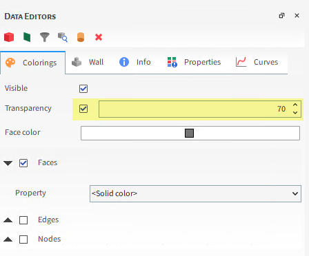
The color, transparency, and visibility of each part of the geometries can be changed from the Coloring tab.
For example, you can make the geometries transparent by doing the following:
1. From the Data panel, under Geometries, multi-select (press the CTRL or SHIFT key while clicking) all 3 of the imported walls.
2. From the Data Editors panel, select the Coloring tab and then enable the Transparency checkbox.
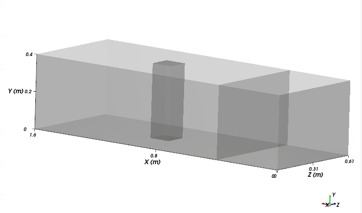
After importing/creating all the necessary geometries, movements can be added using the Motion Frames tool, which is located in the Data panel.
In order to set up a new motion, you will use the following steps:
1. Create a new Frame: You can define a new Frame either setting the position and orientation using the global reference Frame or using a previously created Frame (nested Motion Frame).
2. Define the Frame's motion: Every Frame can have multiple motions defined, which can include:
Translation and Rotation
Vibration and Pendulum
Free Body Translation and Free Body Rotation
Additional Forces and Moments (only for Free Body Motions)
Linear Time Variable Forces and Moments
Time Series (customized) Translation and Rotation
3. Associate the geometry with a Motion Frame: For every moving boundary, select one Motion Frame to be associated with that boundary. To apply a nested set of Motion Frames, assign only the lowest level child Frame.
4. Preview the motion: Use the Motion Preview tool to ensure that the movement for all the boundaries is as desired.
Note: Motion Frames can also be associated with some User Processes.
For this tutorial, one Translation movement will be created for the gate in order to release the water that will be filling the space limited by the container and gate.
To set a Translation Motion, you must either align the Frame with the movement direction, or provide the velocity components. As the gate is aligned to the Y axis, we will provide only the Y velocity for the new frame in order to move the gate upside.
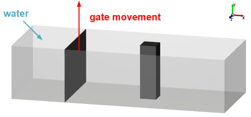
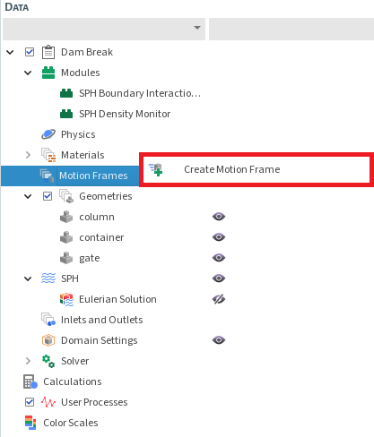
To add a new Motion Frame to your project, do the following:
From the Data panel, right-click Motion Frames, and then select Create Motion Frame.
A new Frame <01> entry appears in the Data panel.
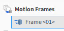
Select the Frame <01> entry to continue setting up the gate movement.
From the Data Editors panel, click the green plus button (Add Motion). A Translation Motion is added by default.
Define Start Time, Stop Time and Velocity (as shown).
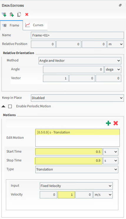
Once the Motion Frame has been created, it can be assigned to the gate geometry.
From the Data panel under Geometries, select gate.
From the Data Editors panel, on the Wall tab, select Frame <01> from the Motion Frame drop-down list.
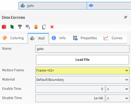
You can check the movement you have just set in a Motion Preview window.
Select Motion Frames from the Data panel.
From Data Editors, click Preview.
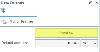
With a Motion Preview window opened, you can use the Time toolbar buttons or slider to visualize the geometry motion.
Tip: The yellow time bar background means that the simulation was not processed yet.
Note: The motion should happen between 0.5 s (initial gate position) and 0.9 s (final gate position), as defined in the Motion Start Time and Stop Time.
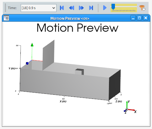
The Materials step allows you to define the Density, thermal (when the thermal model is enabled) and another properties to the SPH and wall geometries.
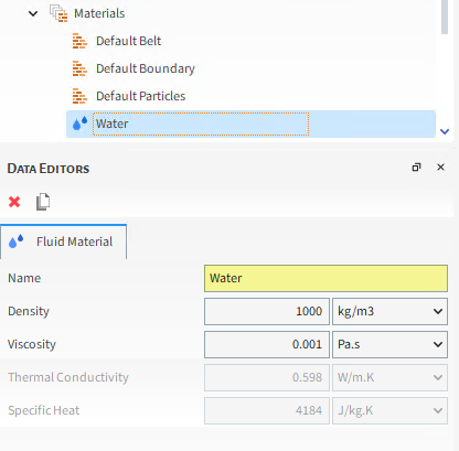
For this tutorial, default values for the boundaries (Default Boundary) will be used and we will set the Fluid Material to represent Water (default values, approximately).
From the Materials entity, select Default Fluid and define the Name in the Data Editors panel.
The SPH step allows you to define which Solver model (WCSPH, IISPH or DFSPH) you will use, and also fluid dynamics, kernel, positions correction and advanced SPH parameters.
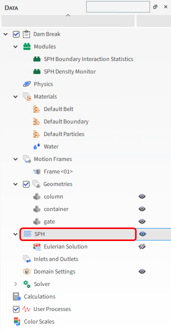
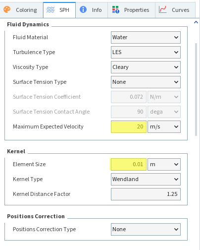
For this tutorial, default values for every parameter but for Element Size and Sound Speed will be used. These last two will be set in order to have consistent results and reduce simulation time.
Note: We are using the IISPH Solver for this tutorial.
From the Data panel, select the SPH entity, and from the Data Editors, on the Model Parameters tab, define the Maximum Expected Velocity and Element Size.
Set your preference color for the fluid (SPH elements) from the Coloring tab on Node color.
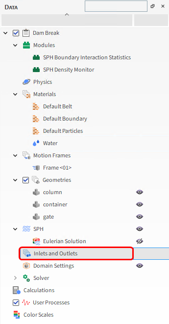
The Inlets and Outlets step allows you to define how fluid enters and exits the simulation. The following options are available:
Fluid Inlet: Releases fluid in a continuous stream from the Surface that you select at a defined Time.
Volumetric Inlet: Fills a prismatic region with SPH elements right before the simulation starts.
Outlet: Defines an Exit Point for fluid to get out of the simulation and allows to define prescribed pressure.
For this tutorial, we will create a Volumetric Inlet to fill part of the container with Water.
1. From the Data panel, right-click Inlets and Outletsand then click Create Volumetric Inlet.
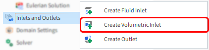
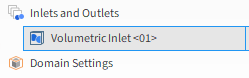
With this, a new Volumetric Inlet <01> entity appears.
From the Data panel, select this new entity.
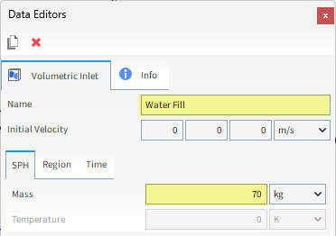
From the Data Editors panel,define the Name and Mass.
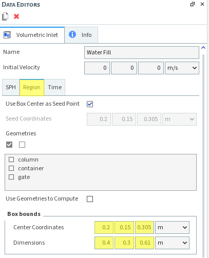
From the Region sub-tab, define Center Coordinates and Dimensions.
In a 3D View it is possible to visualize the region to be filled when Water Fill is selected.
Note: You can also set the dimensions and center of the region with the mouse by clicking and dragging the spheres attached to each face or to the center of the cubic region (for this tutorial, keep the values you defined in the last slide).
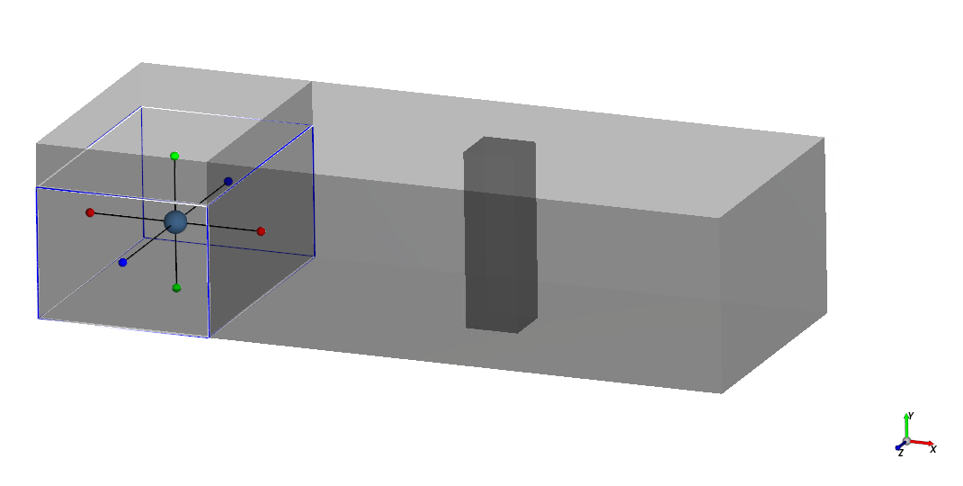
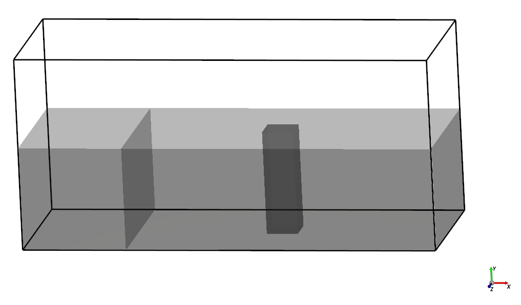
For the Domain Settings step, we will define a custom boundary box that exceeds the limits of our wall geometries.
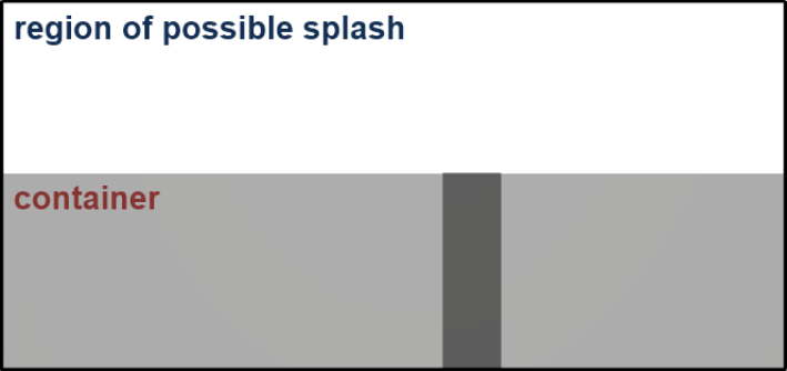
Doing this will allow FreeFlow to compute the elements that possibly escape above the container region (splash from the collision with the column or container).
By default FreeFlow automatically creates a domain box based upon the boundary limits of the Walls.
Any element that leaves those limits is eliminated from the simulation.
These default settings would not work for the dam break simulation as the water splashes over the container region.
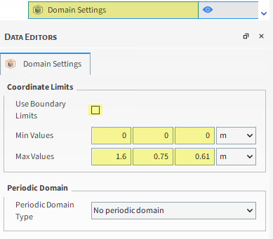
To set the boundary limits:
From the Data panel, click Domain Settings.
From the Data Editors panel, clear the Use Boundary Limits checkbox, and then define the Min Values and Max Values.
View the resulting domain in a 3D View.
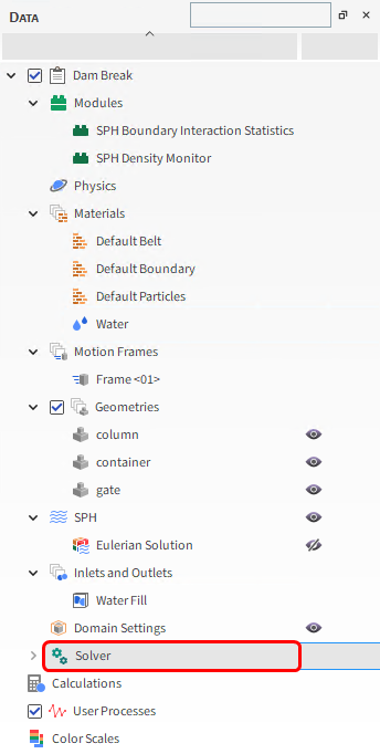
The Solver step is where you define processing time and stability details, and finally Start processing your simulation.
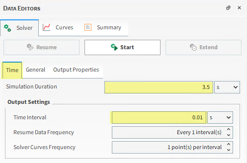
Specifically, the Solver | Time tab is where you define:
Simulation Duration: The total amount of real time that you want the simulation to run.
Output Settings: Time Interval: Time intervals during which you want your output files to be saved.
Output Settings: Solver Curves Frequency: Amount of time between solver Curves updates.
Follow the steps below to set up the solver:
From the Data panel, click Solver, and then from the Data Editors panel, select the Solver | Time tab. Define Simulation Duration and Output Settings | Time Interval.
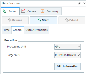
From the General sub-tab, select what you want for Processing Unit, and then the Number of Processors (or Target GPU(s)). For this tutorial, GPU will be faster.
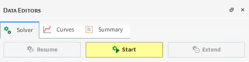
Click the Start button to begin processing.
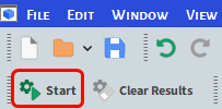
Note: After defining Solver options, it is also possible to begin processing using the Start button from the Simulation Toolbar.
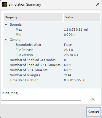
Once you click Start, the Simulation Summary window will appear. It shows the geometry bounds, number of elements and triangles, and the calculated Timestep Duration.
This window will disappear on its own, then processing begins.
While the simulation processes, the program’s title bar shows the number of saved timesteps (Output), the simulated solved time, the real solver time (Elapsed), and the estimated time to finish (ETA).

At the bottom of the screen, you can see the progress bar, the Stop button (to stop the solver), the Refresh button (to visualize the results up to the last solved output), and the Auto Refresh option (to automatically update the 3D View for every newly saved output).
Tip: To view the Fluid state in real time, click the Refresh button or select the Auto Refresh checkbox.

The speed of the simulation depends upon various factors such as:
Number of mesh elements used to define the walls
Smallest element size
Frequency of file output
This completes Part A of this tutorial.
For further information on any topic presented, we suggest searching the User Manual, which provides in-depth descriptions of the tools and parameters.
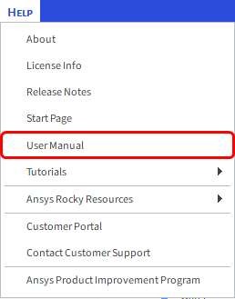
To access this manual, from the main Toolbar click Help, and then click User Manual.
FreeFlow was used to set up and process a dam break simulation.
During this tutorial, it was possible to:
Enable a Module
Import wall Geometries
Define Fluid and Fluid Inlet
Configure the Domain
What's Next?
If you completed this tutorial successfully, then you are ready to move on to Part B and post-process this project.