


When setting up an SPH simulation, you have the option of using the Eulerian Solution feature, which is enabled by default.
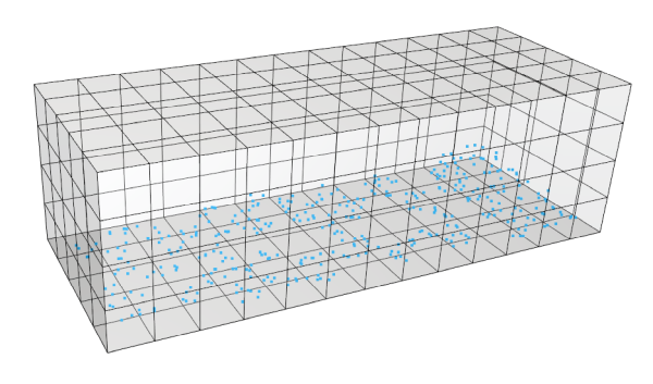
This option allows you to obtain interpolated results of SPH properties onto a fixed Cartesian grid, allowing the use of common visualization and post-processing tools associated to grid discrete representations. (see Figure 3.4: Example of interpolation grid applied to an entire domain. The SPH elements are represented by the blue dots.).
Note: The grid size depends on the domain. Its resolution depends on the selected kernel function and the SPH element size.
Discrete values associated to grid vertices for all relevant flow properties are calculated by using the SPH interpolation expressions including kernel functions.
Figure 3.4: Example of interpolation grid applied to an entire domain. The SPH elements are represented by the blue dots.
This also allows you to analyze specific locations in a simulation where there are no SPH elements in a specific time step. For example, you might use Eulerian Solution to analyze the average density of each individual cell to see at a glance which region of your simulation has a higher fluid density. So while the analysis uses information about the SPH elements, it is actually the individual cells and the simulation locations they represent that are the primary focus.