


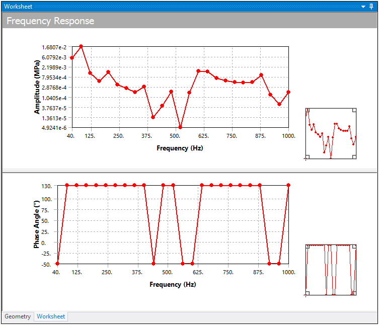
Frequency response results enable you to plot graphs that display how the specified response (stress, strain, etc.) varies with frequency. You can view these responses as a value graphed along a specified frequency range. Plots include all the frequency points at which a solution was obtained. When you generate frequency response results, the default plot (Bode) shows the amplitude and phase angle. You can parameterize frequency results.
Go to a section topic:
Application
Select the Solution object and then select a desired result from the Frequency Response drop-down menu on the Solution Context tab. You can also use the context (right-click) menu on the Solution object or from within the Geometry window and select > Frequency Response > [Result Type]. Menu options include:
Specify the properties of the In the Details pane for the object. The availability and selections of the properties vary based on the result type you specify. See the Property Definition topic below for more information.
Property Definition
The Details pane properties for this result include the following.
| Category | Properties/Options/Descriptions |
|---|---|
|
Contribution[a] |
Panel Contribution: This property enables you to visually compare the results of one or more solid bodies as a mosaic chart. You use this feature to create a "panel" for each body included in your model. However, you can only scope the supported result to the faces of a body, using either geometry or Named Selection. Using these faces, the application calculates results for each panel (body) included in the face-based scoping. Options include (default) and . Mode Contribution: This property enables you to visually compare results from one or more modes using a mosaic chart. You use this feature to highlight the contributions of selected modes for your results. Mode contribution analysis can be applied to any geometry or named selection, including nodes, surfaces, and bodies. Options include (default) and . |
|
Scope[b] |
Scoping Method: Based on the selected result, supported Scoping Method property options include:
Load Step Number: This property is visible when the Multiple Steps property is set to and the Multiple Step Type property is set to Load Step (default). Both of these properties are available in the Analysis Settings > Step Controls category. Specify a desired load step. The default setting is 1. RPM Selection: This property is visible when the Multiple Steps property is set to and the Multiple Step Type property is set to . Both of these properties are available in the Analysis Settings > Step Controls category. Select a RPM value from the drop-down menu. Spatial Resolution: This property enables you to specify which solution data to use for the calculation of the result for the given scoping, either the averaged result values or the minimum or maximum values. Options include Use Average (default), Use Minimum, and Use Maximum. The Use Average setting calculates the average by calculating the real and imaginary components separately. The Use Minimum and Use Maximum options are based on amplitude and report. Note:
|
|
Definition |
Type: This property identifies the result type, as listed below, you selected the Frequency Response drop-down menu. It provides either a drop-down menu to further define the Stress or Strain results or it is a read-only value of the selected result type.
Orientation: Specify the orientation in which results are to be extracted. Options include , , and . Coordinate System: Specify a desired coordinate system. Options include Global Coordinate System, Solution Coordinate System, and any available local coordinate systems you define. Suppressed: Include or exclude the object during the analysis. Options include and (default). |
|
Frequency Filter: Use this entry property to further filter graph and tabular data by frequency value. The frequency value displays the selected unit system, however, in order to reflect a change to the unit system in a resumed model, you must manually re-enter or update the value. The default option is . Display Panel: Only visible when the Panel Contribution property is set to . Use this property to view the mosaic chart referencing the panel contribution. Options include and (default). When you set this property to Yes, the following additional properties display:
| |
|
Options |
See the Results and Result Tools (Group) object reference page for property descriptions. |
|
Results |
See the Results and Result Tools (Group) object reference page for property descriptions. |
[a] Only available for the Deformation, Velocity, and Acceleration result types.
[b] The and result types do not include this category.
[c] Equivalent radiated power results estimate the radiated structure-borne sound power from a vibrating structural surface. These results are available in 3D Harmonic Response and Harmonic Acoustics (if you define a structural Physics Region) analyses. The result is evaluated on faces that you select, either using face geometry section or face-based Named Selections, and the result is displayed on a graph over the specified frequency range. You specify the frequency range using the setting for the Frequency Range property. When you generate frequency response results, the plot shows Equivalent Radiated Power (ERP) or Equivalent Radiated Power Level (ERPL) as a function of the frequency. See the expressions described below as well as the PLAS command for the ERP and ERPL acoustic quantities.
Requirement: Equivalent Radiated Power and Equivalent Radiated Power Level results must be scoped to either surfaces or element faces.
Important: For Equivalent Radiated Power and Equivalent Radiated Power Level results, if the Multiple Step Type property is set to in the Analysis Settings, the result file must exist for the result to be displayed.
Note:
You can specify a weighting filter (A, B, and C) for the Equivalent Radiated Power Level result.
For the Equivalent Radiated Power (ERP) and Equivalent Radiated Power Level results, when the On Demand Expansion Option property is set to , the application always calculates the Minimum/Maximum values displayed in the Results category of the Details pane based on the Frequency Range specified in the Analysis Settings. The application does not filter them based on the Frequency Range specified in the result object. This filtering only applies to the Charts, Graph, and Tabular Data.
Limitations
If the Store Results At All Frequencies property in the Options category of the Analysis Settings is set to , the Frequency Response results for force reactions cannot be extracted.
Result Calculation Descriptions
The following equations describe how frequency graphs are defined and plotted for the supported types.
- Stress and Strain Results
The strain result is calculated using the displacement result. Using the Young’s Modulus and strain result, the stress result can be evaluated. Because of this reason, the stress and strain results are in phase with the displacement result.
- Deformation Result
The displacement vector on a structure subjected to harmonic loading may be expressed as:
EQUATION 1

The Frequency Response chart for displacement is calculated by expressing Equation (1) in time domain as follows:
EQUATION 2

where:


- Velocity Result
The equation for velocity
 can be obtained by taking a time derivative of Equation (1). The
frequency response for velocity in time domain is calculated as follows:
can be obtained by taking a time derivative of Equation (1). The
frequency response for velocity in time domain is calculated as follows:EQUATION 3

where:


- Acceleration Result
The equation for acceleration
 can be obtained by taking a double time derivative of Equation (1).
The frequency response for acceleration in time domain is calculated as follows:
can be obtained by taking a double time derivative of Equation (1).
The frequency response for acceleration in time domain is calculated as follows:EQUATION 4

where:


- Force Reaction
The Frequency Response for Force Reaction is calculated by replacing displacement with force in Equation (2) as shown below.
EQUATION 5

where:


 (Amplitude)
 (Phase Angle)
- Equivalent Radiated Power
Equivalent Radiated Power (ERP) is expressed as:

Where:
 = speed of sound (equal to 343.25 m/s).
 = mass density (equal to 1.2041 kg/m3).
 = radiation factor (equal to 1).
 = normal velocity of vibrating structural surface
 - Equivalent Radiated Power Level
The Equivalent Radiated Power Level (ERPL) is expressed as:
ERPL = 10 Log (ERP/Wref) Where Wref is the reference sound power (equal to 10-12W).
- Krylov Residual Norm
This result plots error estimations (residuals) across a frequency range for the harmonic distribution. The result displays the lowest residual value at the frequency where the Krylov subspace is built. High residual values indicate the error between the actual and the approximated solution for a given high frequency. The plot can provide information on how to best split the whole frequency range into multiple ranges. The Krylov Residual Norm is calculated using the following equation:

Where:
 is the applied force.
 is the approximated force using the Krylov method.
For  , K, M, and C are the system matrices and the Residuals are
calculated for all the solved frequency points
ωi.
, K, M, and C are the system matrices and the Residuals are
calculated for all the solved frequency points
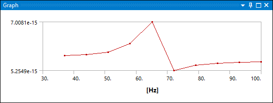
ωi.Example Plot
Display Options
- Display Property
The Display Property property of the frequency response results provides the following results values for graphs:
(default setting - plots both Amplitude and Phase Angle)
- Chart Viewing Style Property
The Chart Viewing Style property provides the following options to plot results for a scale of an axis:
: this option plots the result values linearly.
: this option plots the X-Axis logarithmically. If negative axis values or a zero value exists, this option is not supported and the graph plots linearly.
(default when graph has Amplitude): this option plots the Y-Axis is plotted logarithmically. If negative axis values or a zero value exists, this option is not supported and the graph plots linearly.
: this option plots the X-Axis and Y-Axis logarithmically. If negative axis values or a zero value exists, this option is not supported and the graph plots linearly.
Note: You cannot use the Mechanical application convergence capabilities for any results item under a harmonic analysis. Instead, you can first do a convergence study on a modal analysis and reuse the mesh from that analysis.
Presented below is an example of a Frequency Response plot:
The average, minimum, or maximum value can be chosen for selected entities. Stress, Strain, Deformation, Velocity, and Acceleration components vary sinusoidally, so these are the only result types that can be reviewed in this manner. (Note that items such as Principal Stress or Equivalent Stress do not behave in a sinusoidal manner since these are derived quantities.)
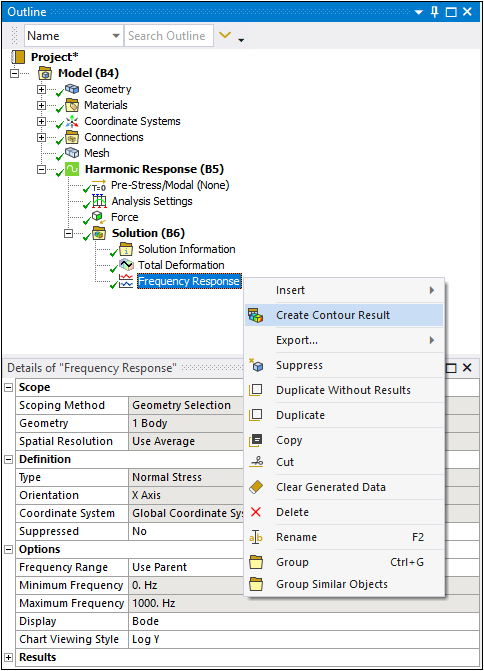
Create Contour Results from Frequency Response Results
You can use Frequency Response result types (not including Velocity and Acceleration) to generate new result objects of the same type, orientation, frequency. The phase angle of the contour result will be opposite in sign with the same magnitude as the frequency response result type. The sign of the phase in the Sweeping Phase property of the contour result is reversed so that the response amplitude of the frequency response plot for that frequency and phase defined by the Duration property matches with the contour results. To create a Contour Result in a Harmonic Analysis:
Select and right-click the desired Harmonic result in the solution tree.
Choose .
As illustrated here, you can see how the feature automatically scopes the Type, Orientation, Coordinate System, Frequency, and Sweeping Phase.
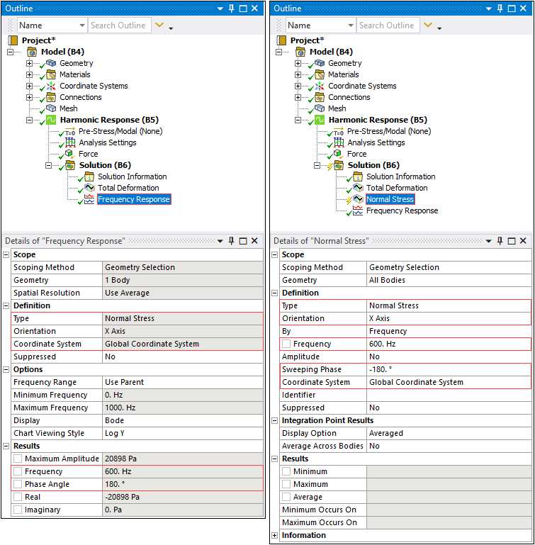
The Reported Frequency in the Information category is the frequency at which contour results were found and plotted. This frequency can be potentially different from the frequency you requested.