


This tutorial includes:
This tutorial teaches you how to:
Import hub, shroud, and blade geometry from individual curve files.
Change the method of constructing the hub and shroud curve types.
Make colored surfaces to show variations in mesh measures (such as
Minimum Face Angle).Add a blade blend made using the rolling ball process with a constant radius (BladeModeler or BladeBuilder license required).
As you work through this tutorial, you will create a mesh for a blade passage of a steam stator. A typical blade passage is shown by the black outline in the figure below.
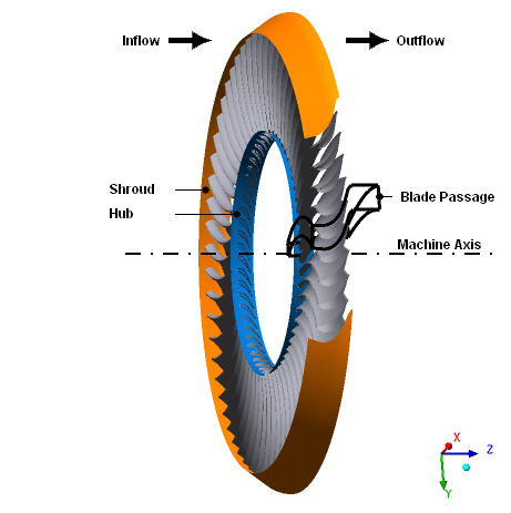
The stator contains 60 blades distributed about the Z axis. A clearance gap exists between the blades and the shroud, with a width of 2% of the total span. Within the blade passage, the maximum diameter of the shroud is approximately 97.5 cm.
If this is the first tutorial you are working with, it is important to review Introduction to the Ansys TurboGrid Tutorials before beginning.
Create a working directory.
TurboGrid uses a working directory as the default location for loading and saving files for a particular session or project.
Download the
stator.zipfile here .Unzip
stator.zipto your working directory.Ensure that the following tutorial input files are in your working directory:
BladeGen.inf
shroud.curve
hub.curve
profile.curve
Set the working directory and start TurboGrid.
For details, see Setting the Working Directory and Starting Ansys TurboGrid.
In the first tutorial, you loaded a BladeGen.inf file in order to specify the machine data (# of blade sets,
rotation axis, and units) and curve files. In this tutorial, you will
enter such data manually using the Load Profile Points Or CAD command.
Load the curve files for the steam stator as follows:
Click File > Load Profile Points Or CAD.
The geometry browser (the main object editor of the Geometry workspace) appears. TurboGrid fills in the names of the curve files based on the files that are present in the working directory; The first
.crvor.curvefile found that has a name containing “hub”, ”shroud”, or “blade”/”profile” is selected as the hub, shroud, or blade file, respectively.Ensure that, under Point Data Definition > TurboGrid Curve Files, Hub is set to
./hub.curve, Shroud is set to./shroud.curve, and Blades is set to./profile.curve.Set Point Data Definition > Coordinates and Units > Coordinates to
Cartesianand Length Units tocm.These units are used to interpret the data in the curve files.
Set Geometry Setup > Rotation > Method to
Principal Axisand Axis toZ.Set Geometry Setup > # of Bladesets to
60.Click to save the settings.
Return to the Mesh tab to view the geometry.
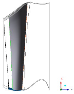
The progress bar at the bottom right of the screen shows the geometry generation progress. After the geometry has been generated, you can see the hub, shroud, and blade for one passage. Along the blade, you can see the leading and trailing edge curves (green and red lines, respectively). Near the blade, you can see the inlet and outlet markers (white octahedrons).
Rotate the geometry into the position shown in Figure 3.1: Incorrect Hub and Shroud Representations.
As shown in Figure 3.1: Incorrect Hub and Shroud Representations, the hub and shroud are greatly distorted. This is the result of using spline curves to construct the hub and shroud based on relatively few data points. This problem will be corrected in the next section.
Set the method of constructing the hub and shroud as follows:
Open
Geometry>Hub.Set Geometric Representation > Curve Type to
Piece-wise linear.Click Apply.
Set
Shroudin the same way.
To complete the geometry, create a small gap between the blade and the shroud. The blade should be shortened to 98% of its original span because the gap width is 2% of the total span, as specified in the problem description.
Open
Geometry>Blade Set>Shroud Tip.Set Tip Option to
Constant Span.Set Span to
0.98.Click Apply.
This completes the geometry definition.
Click Hide all geometry objects
 to turn off the visibility of the geometry.
Right-click
Topology Setand turn off Suspend Object Updates.After some time, you will see a warning message about the inlet domain being turned off.
Dismiss the warning message.
The topology and 3D mesh are generated.
Turn on the visibility of
Layers>Hubto show the topology on the hub.Turn on the visibility of
Layers>Shroud Tipto show the topology on the shroud tip.
Note: It might be useful to keep the same topology when studying a range of blade geometries, or the same blade on different computers. To keep the same topology, use the Manual (Advanced) setting for the topology. This setting is available after clicking Edit > Options and selecting Enable Advanced Features.
TurboGrid automatically computes a default mesh and sets the base mesh dimensions.
Each unique mesh dimension has an edge refinement factor that
is multiplied by the base mesh dimension and global size factor to
determine the final mesh size. The overall mesh size is controlled
using the Method setting in the Mesh
Data object editor on the Mesh Size tab. Setting the Method to Target
Passage Mesh Size enables you to specify a Node
Count. Using this method specifies an approximate mesh
size (in nodes) and lets TurboGrid compute the mesh dimensions automatically.
Setting the Method to Global Size Factor enables you to specify a Size Factor. Increasing
this factor will increase the overall mesh size, and decreasing it
will decrease the overall mesh size. The change is nonlinear.
The Boundary Layer Refinement Control settings affect the mesh in the O-Grid region around the blade:
Note that, when Boundary Layer Refinement Control > Method is set to
Proportional to Mesh Size, the number of elements across the boundary layer is calculated as Base Count * Global Size Factor * (Factor Base + Factor Ratio * Global Size Factor). The default values of Factor Base and Factor Ratio are 3 and 0 respectively.The Target Maximum Expansion Rate setting affects the expansion rates that are used just outside the blade profile.
The Near Wall Element Size Specification settings control the method by which the near-wall node spacing is specified on the Passage, Hub Tip, and Shroud Tip tabs. The near-wall node spacing is the distance between a wall (for example, hub, shroud, or blade) and the first layer of nodes from the wall. The Method setting has these options:
Y Plus — The
y+method sets the near-wall spacing to a target value, y+, in relation to a set Reynolds number.Absolute — The
Absolutemethod enables you to set the near-wall spacing directly on the Passage, Hub Tip, and Shroud Tip tabs.
The Inlet Domain and Outlet Domain check boxes enable you to generate the inlet and outlet domains as part of the mesh. Settings that affect these grid regions are found on the Inlet/Outlet tab.
Selecting the Lock mesh size check box forces the total number of nodes and elements to remain constant.
On the Shroud Tip tab, you can use the Blade Tip > Override Target Maximum Expansion Rate setting to override the Target Maximum Expansion Rate value set on the Mesh Size tab, to govern the expansion rate of elements that cross the tip mesh.
If the topology were grossly skewed or distorted on the hub
or shroud layer, the Layers object would be shown
with red text in the object selector. Since the Layers object is shown in black text, the mesh contains no regions with
high skew on the hub or shroud.
By default, TurboGrid automatically generates the recommended number of layers
before the mesh is generated. This default behavior can be disabled by editing the
Layers object so that Insertion Mode is not set to
Automatic - Adaptive.
A turbo surface of constant "K" (a nodal coordinate) appears. This surface is
listed in the object selector as 3D Mesh > Show Mesh.
You can change the location and coloring of this surface to explore the mesh.
Check the 3D mesh statistics:
Open
Mesh Analysis.The mesh statistics are acceptable based on the current quality criteria.
Close the Mesh Statistics dialog box.
The predefined surfaces found under the 3D Mesh object in the object selector are useful for showing variations
in the mesh statistics.
In the following section, you will color 3D Mesh > Show Mesh by Minimum Face Angle. You will then create a legend for that object.
Turbo Surfaces can be created by selecting Insert > User Defined > Turbo Surface. In this case, you will simply edit the predefined turbo surface.
Open
3D Mesh>Show Mesh.Leave Variable, and Value unchanged.
Click the Color tab and set Mode to
Variable.Set Variable to
Minimum Face Angle.Set Range to
Local.This will cause the range of colors in the color map to be distributed over the range of values found on the turbo surface, rather that over the global range or a user-defined range.
Click the Render tab.
Ensure that Draw Faces is selected.
Click Apply to apply the changes to the turbo surface.
To illustrate the scale of the Minimum Face Angle variable, create a
legend for the turbo surface:
Click Insert > User Defined > Legend.
Click to accept the default name.
Set Plot to
TURBO SURFACE:Show Mesh.Set Title Mode to
Variable and Location.Click Apply to create the legend.
In this section of the tutorial, you will add a blade blend (fillet) using the blade blend object. A blade blend object specifies hub and/or shroud blends (fillets) made by the rolling ball process with a constant radius.
Note: The blade blend object makes use of the CAD From Profile Points input mode, which, in general, requires either
a BladeModeler license or a BladeBuilder license. This tutorial happens to use BladeEditor as a CAD generator, so requires
a BladeModeler license.
The CAD From Profile Points input mode is available only in stand-alone mode; it is not
supported in Ansys Workbench.
Add a blade blend object as follows:
In the Mesh workspace, right-click
Blade 1and select Insert > Blade CAD Feature > Blade Blend.The Blade CAD Features object editor opens with the Blade Blends tab displayed.
In the object editor, select Hub Blend and set Hub Blend > Rolling Ball Radius to
2.5 [mm].Click Apply.
(Do not click Apply And Generate CAD because you will review settings in the geometry browser before generating CAD.)
In the Geometry workspace, in the geometry browser:
On the Input Selection tab, set Input Mode to
CAD From Profile Points.The CAD Properties tab appears.
On the CAD Properties tab, ensure that Blend Style is set to
Approximate Blend (Low Fidelity Geometry Only)and that CAD Generation Tool > Tool is set toBladeEditor.Note that the default tool is specified by a user preference.
Click Apply And Generate CAD.
TurboGrid drives Ansys BladeModeler in the background to generate CAD geometry.
The geometry is now entirely represented by CAD that was generated, using Ansys BladeModeler, based on the profile point definition (provided by curve files) and the blade blend specification (provided by the blade blend object).
If there is any change to the curve files or blade blend object, be sure to regenerate the geometry. You can regenerate the geometry from the Apply and Generate CAD button or from File > Update Geometry. In particular, even after loading a state file, you might need to regenerate the geometry if the profile point definition or blade blend specification has changed since the last time the CAD geometry was generated.
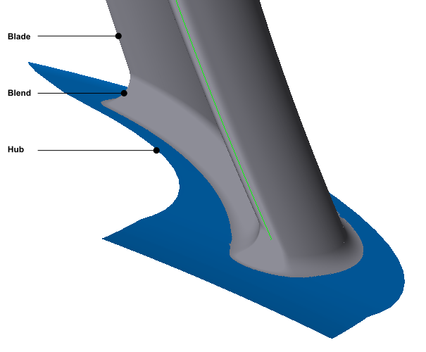
The blade blend is shown in Figure 3.2: Blade Blend Shown.
Note: A known issue with using the blade blend object can result in failure of CAD generation. If CAD generation fails, try making a very small change to the blend radius.
Other troubleshooting alternatives:
Specify the
Layersobject with Insertion Mode set toAutomatic - Adaptive.Specify the
Layersobject with Insertion Mode set toManual - Uniform.Specify the
Topology Setobject with Mesh Generation Mode set toATM3D.
Save the mesh:
Click File > Save Mesh As.
Ensure that Files of type is set to
Ansys CFX Mesh Files.Set Export Units to
cm.Set File name to
steam_stator.gtm.Ensure that your working directory is set correctly.
Click Save.