


This tutorial includes:
- 5.1. Preparing the Working Directory
- 5.2. Defining the Geometry
- 5.3. Creating the Topology and Mesh
- 5.4. Decreasing the Mesh Density
- 5.5. Observing the Mesh
- 5.6. Using the Locking Feature
- 5.7. The Y+ Functionality
- 5.8. Using Local Mesh Refinement
- 5.9. Analyzing the Mesh
- 5.10. Adding Inlet and Outlet Domains
- 5.11. Analyzing the New Mesh
- 5.12. Saving the Mesh
- 5.13. Saving the State (Optional)
This tutorial teaches you how to:
Switch to a Meridional (A-R) projection in the viewer.
Change the shape and position of the
InletandOutletgeometry objects that bound the blade passage in the streamwise direction.Use Local Mesh Refinement
Extend the mesh by adding inlet and outlet domains.
As you work through this tutorial, you will create a mesh for a blade passage of a fan. A typical blade passage, inlet domain, and outlet domain, are shown by the black outline in the figure below.
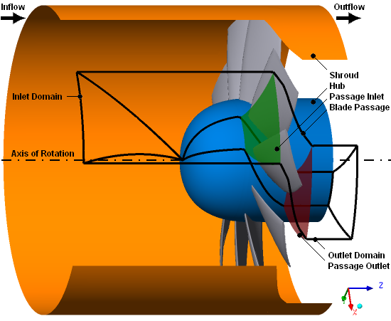
The fan contains 10 blades that revolve about the negative Z axis. A clearance gap exists between the blades and the shroud, with a width of 2% of the total span. The shroud diameter is approximately 26.4 cm.
Let the mesh contain an inlet domain and an outlet domain.
If this is the first tutorial you are working with, it is important to review Introduction to the Ansys TurboGrid Tutorials before beginning.
Create a working directory.
Ansys TurboGrid uses a working directory as the default location for loading and saving files for a particular session or project.
Download the
fan.zipfile here .Unzip
fan.zipto your working directory.Ensure that the following tutorial input files are in your working directory:
BladeGen.inf
shroud.curve
hub.curve
profile.curve
Set the working directory and start Ansys TurboGrid.
For details, see Setting the Working Directory and Starting Ansys TurboGrid.
To obtain the basic geometry, you will load a BladeGen.inf file. After inspecting the geometry and improving the shape of the
inlet and outlet, you will finish defining the geometry by creating
the required gap between the blade and the shroud.
Load the BladeGen.inf file, then inspect
the geometry by viewing it in axial-radial coordinates:
Click File > Load TurboGrid Init File.
Open
BladeGen.inffrom the working directory.In the Mesh workspace, right-click a blank area in the viewer, and click Transformation > Meridional (A-R) from the shortcut menu.
The passage inlet, which appears in the object selector as Geometry > Inlet, is the upstream
end of the blade passage (but not necessarily the upstream end of
the mesh, since, as you will see in this tutorial, you can add an
inlet domain upstream of the passage inlet). The passage inlet is
generated by revolving a curve, which is defined in an axial-radial
plane, about the machine axis. That curve, in turn, is generated according
to a set of points, known here as inlet points. These points appear as white octahedrons in the viewer. The passage
outlet is analogous to the passage inlet, and is downstream of the
blade passage.
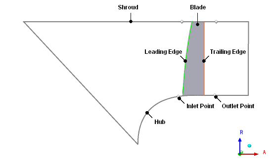
Notice that, in this case, there are two inlet points and they are located at different distances from the blade. In order to obtain a high-quality mesh topology for the blade passage, the inlet points should be repositioned.
Reposition the inlet and outlet points as follows, and observe the movement of the inlet and outlet points in the viewer:
Open
Geometry>Inlet.Select Interface Specification Method > Points.
Select
Low Hub Point, then set Method toSet Aand Location to-0.008.Click Apply.
Select
Low Shroud Point, then set Method toSet Aand Location to0.002.Click Apply.
Open
Geometry>Outlet.Select Interface Specification Method > Points.
Select
Low Hub Point, then set Method toSet Aand Location to0.03.Click Apply.
Select
Low Shroud Point, then set Method toSet Aand Location to0.03.Click Apply.
To complete the geometry, create a small gap between the blade and the shroud. The blade should be shortened to 98% of its original span because the gap width is 2% of the total span, as specified in the problem description.
Open
Geometry>Blade Set>Shroud Tip.Set Tip Option to
Constant Span.Set Span to
0.98.Click Apply.
Right-click a blank area in the viewer and select Transformation > Cartesian (X-Y-Z) from the shortcut menu.
Click Hide all geometry objects
 .
.This gives you an unobstructed view of the topology, and later the mesh.
Right-click
Topology Setand turn off Suspend Object Updates.Turn on the visibility of
Layers>Hubto show the topology on the hub.Turn on the visibility of
Layers>Shroud Tipto show the topology on the shroud tip.
The topology and 3D mesh are generated.
Note: Mesh quality issues are discussed later in this tutorial.
There are several ways to control the mesh size:
Changing the global size factor.
Using proportional refinement in the boundary layer.
Changing the number of mesh elements in the spanwise direction in the passage.
Changing the edge refinement on a specific edge, including within the boundary layer.
Begin by changing the global size factor and the amount of refinement in the boundary layer:
Open
Mesh Data.On the Mesh Size tab, set Method to
Global Size Factor.Set Size Factor to
0.9.An overall decrease in mesh size can be useful in reducing the computational resources required for simulation.
Ensure that Boundary Layer Refinement Control > Method is set to
Proportional to Mesh Size.Set Factor Base to
2.6.Click Apply.
Observe that the number of nodes has been reduced and the element size has increased in the boundary layer mesh. With proportional refinement enabled, the relationship between the height of the first element in the boundary layer and the global size factor should be approximately inversely proportional (that is, an increase in the global size factor will cause a decrease in the element height).
Right-click a blank area in the viewer, and select Predefined Camera > Isometric View (X Up).
A K-Plane is displayed by default. This shows the 2D mesh on a layer. The plane can be moved in the spanwise direction by holding Ctrl + Shift and dragging using the left mouse button.
Turn on the visibility of the following objects under
3D Mesh:HIGHBLADE GEO HIGHHIGHBLADE GEO LOWHUBLOWBLADE GEO HIGHLOWBLADE GEO LOWSHROUDShow Mesh
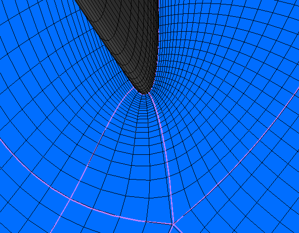
Note that the mesh element density is higher near the blade and hub, as can be seen in Figure 5.1: Mesh at Blade-Hub Intersection.
The number of mesh elements in the spanwise direction is automatically changed depending on the global size factor and the mesh element size at the boundary layer.
Next, increase the mesh size in the spanwise direction by a factor of 1.5:
Open
Mesh Data.On the Passage tab, set Spanwise Blade Distribution Parameters > Method to
Proportionaland Factor to1.5.Note that the disabled # of Elements field indicates the total number of elements in the spanwise direction. This will now increase.
Click Apply.
The number of elements has increased.
Note: This section is for information only. Do not use the locking feature in this tutorial.
When you are using Ansys Workbench, Ansys TurboGrid enables you to use the Lock mesh size feature. Once activated, the total number of nodes and elements will remain constant. This holds true even if the geometry of the blade is changed. The size of the mesh elements will be readjusted, but the total number will not be changed. The Lock mesh size check box is in the Mesh Data object editor on the Mesh Size tab.
Another method of controlling the mesh size at the boundary layer is specifying the y+ height and Reynolds number. This option lets you specify the maximum y+ height for the blade, which is then used to calculate the edge refinement factor. The actual first element offset will not be consistent across the boundary layer, although it should be equal or less than the maximum specified. The edge refinement calculation is only an approximation.
You will enable the option for y+, then set the offset to 15. You will also set the Reynolds number to 500,000.
Open
Mesh Data.On the Mesh Size tab, set Boundary Layer Refinement Control > Near Wall Element Size Specification > Method to
y+.Set Reynolds No. to
5e5.Change Boundary Layer Refinement Control > Method to
First Element Offset.The field for specifying Offset Y+ is enabled.
Set Parameters > Offset Y+ to
5.Click Apply.
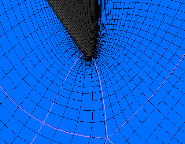
You should see an increase in the mesh density at the boundary layer.
The mesh now has smaller elements near the boundary layer, as shown in in Figure 5.2: Mesh at Blade-Hub Intersection After Y+ Specification.
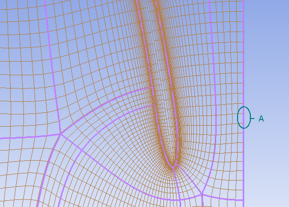
Local mesh refinement is especially useful when attempting to manipulate the mesh near a specific boundary without tampering with the surroundings. Once local mesh refinement has been implemented, changing the global size factor will affect the localized area as well. However, the locally refined mesh will remain discernible from its surroundings. You will implement this feature at the shroud boundary, upstream of the blade as indicated in the figure below. The local mesh size will be increased by 100%.
Click Hide all mesh objects
 .
.To be able to see which boundary to modify, it is best to hide the currently generated mesh. Ultimately, only the topology will be visible when refinements are made.
Right-click a blank area in the viewer and select Predefined Camera > View from +X from the shortcut menu.
Turn off the visibility of
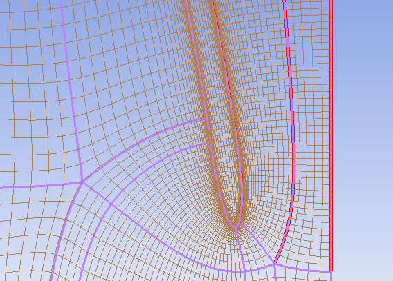
Layers>Hub.Right-click the edge of the shroud tip layer, marked A in Figure 5.3: Edge to be Refined in Shroud Tip Layer, and select Increase Edge Refinement > 100%.
After a few seconds of processing, you should observe the mesh size increasing by a factor of 2 at the edge you selected. Only topologically parallel edges are affected by this change.
Inspect the mesh quality of the 3D mesh:
Open
Mesh Analysis.The mesh statistics are acceptable based on the current quality criteria.
Close the Mesh Statistics dialog box.
As specified in the problem description, the mesh should contain an inlet domain and an outlet domain.
Open
Mesh Data.On the Mesh Size tab, ensure that Inlet Domain and Outlet Domain are selected.
Click Apply.
Open
Mesh Analysis.Note that the
Edge Length Ratiomesh measure is extremely large. By displaying this mesh measure, you will see that some of the mesh elements that exceed the criterion are at the inlet where the mesh meets the rotation axis. This is to be expected wherever the hub reaches the axis of rotation because at these locations the element edges have zero length.View the mesh on the inlet and outlet (not the passage inlet and outlet, but the inlet and outlet of the entire mesh) by turning on the visibility of the corresponding
3D Meshobjects.
Save the mesh:
Click File > Save Mesh As.
Ensure that Files of type is set to
Ansys CFX Mesh Files.Set Export Units to
cm.Set File name to
fan.gtm.Ensure that your working directory is set correctly.
Click Save.