


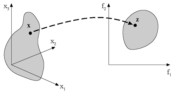
Most real-world optimization problems include more than one objective and a large number of design variables. This leads to the general formulation of the multi-objective optimization problem
 | (4–33) |
with  as the vector of design variables and the constraints of inequality
 and equality
  . All solutions which comply with both constraints and variable bounds form the
feasible
. All solutions which comply with both constraints and variable bounds form the
feasible  -dimensional design space. Each solution
  is assigned to a vector
  describing one point of the
  -dimensional objective space. This is the major difference to the
single-objective optimization problem where there is only one objective. The mapping between
design space and objective space is illustrated in Figure 4.26.
-dimensional objective space. This is the major difference to the
single-objective optimization problem where there is only one objective. The mapping between
design space and objective space is illustrated in Figure 4.26.
Several procedures have been developed to solve a multi-objective optimization problem (Branke et al. 2008). They are classified in non-interactive and interactive methods. In non-interactive methods the multi-objective optimization problem is transferred into a singe-objective problem. This can be done e. g. by choosing a preferred objective function and introducing the remaining objectives as constraints (see Section 4.3.3)
 | (4–34) |
Another possibility is to combine all objectives in a single function by using individual
weights  (see Section 4.3.2):
 | (4–35) |
Both methods require good knowledge about the optimization potential with respect to each objective function and a clear idea about the importance of the different objectives with respect to each other.
In early stages of the design process such information are often rare and a transformation of the multi-objective task into a single objective task is not possible a priori. In such cases interactive methods are more promising. In optiSLang Pareto optimization as one of the most popular interactive methods is available.
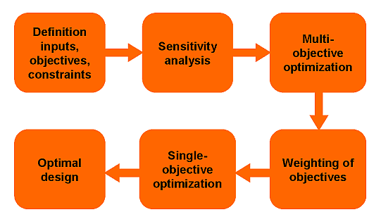
In Figure 4.27 the recommended flow for a multi-objective optimization procedure is shown: initially the inputs, possible objectives and constraint functions are defined. Sensitivity analysis is used to detect unimportant parameters and to check the objective functions with respect to possible conflicts. Afterwards, a multi-objective optimization is performed to determine the optimization potential within the conflicting objectives and to derive suitable weighting factors for a following single-objective optimization. Finally this single-objective optimization determines an optimal design.
References
Branke, J., K. Deb, K. Miettinen, and R. Slowinski. 2008. Multiobjective Optimization. Springer.
Solving the multi-objective optimization problem requires a criterion which regards the
distinct objectives. One possible criterion is the Pareto dominance which is formulated for
two decision vectors  and
and  in the design space
  as follows
Solution
 dominates solution
  if it is feasible and better or equal in all objectives and better in at
least one objective.
if it is feasible and better or equal in all objectives and better in at
least one objective. Solution
 is indifferent to solution
  if none of both solutions dominates the respective other.
Figure 4.28: Pareto dominating (filled circles) and dominated designs (unfilled circles) including
the resulting Pareto frontier of two conflicting objectives. ( and
and  dominate
  but are indifferent to each other)
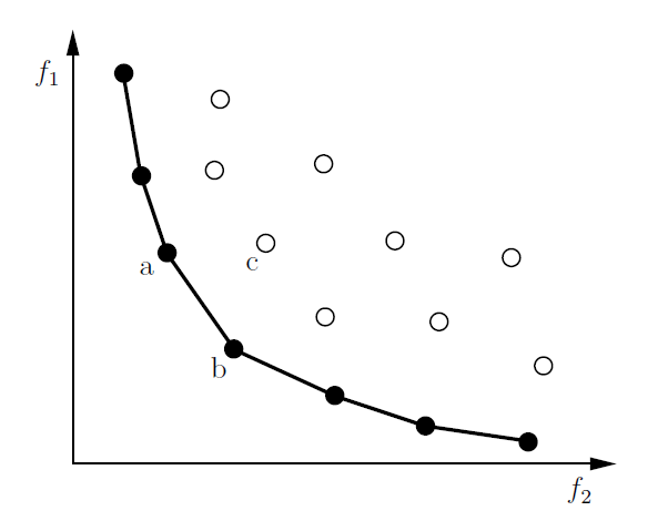
Using the dominance criterion allows for creating a partial order between different decision vectors as illustrated in Figure 4.28. A solution is Pareto optimal if there is no decision vector that would improve one objective without causing a deterioration in at least one other objective. In other words a solution is Pareto optimal if it is not dominated by any other solution. The term Pareto is named after Vilfredo Pareto, an Italian economist who used the concept in his studies of economic efficiency and income distribution.
If all objectives are equally important and no preferences are made a priori, the dominance of a solution is the only way to determine if it is better than others. As a result the non-dominated subset out of the feasible set of solutions constitutes the Pareto set. The corresponding points in the objective space are called Pareto frontier. The following requirements concerning the multi-objective optimization can be formulated:
Find a set of solutions close to the Pareto optimal solutions (convergence).
Find solutions which are diverse enough to represent the whole Pareto frontier (diversity).
Although the optimization produces a set of Pareto optimal solutions, the user is interested in getting only one solution. Additional preferences have to be introduced, which needs comprehensive knowledge about the problem, to select a solution that meets the requirements.
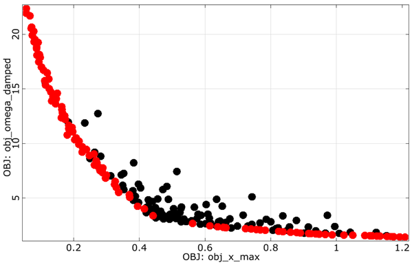
In order to obtain different trade-off solutions there must be conflicting objectives. The results of a preceding sensitivity analysis should be used to check the objective functions concerning possible conflicts.
Figure 4.29: Conflicting objectives of the damped oscillator (maximum amplitude vs. eigen-frequency) including cluster analysis of the Pareto optimal designs in the objective space (left) and in the design space (right)
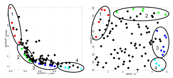
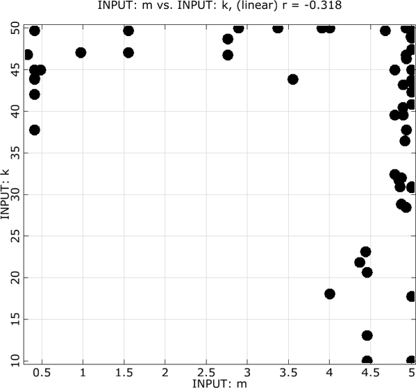
In case of the oscillator example the damped eigen-frequency is used as second objective function which should be minimized. The anthill plots of the samples used for the sensitivity analysis and design exploration are shown in Figure 4.29. The figure indicates that the minimization of the maximum amplitude is in conflict with the minimization of the damped eigen-frequency. In the anthill plot all Pareto dominant designs can be identified. Further information can be gained by subdividing the Pareto optimal designs in the objective space in clusters which are investigated with respect to their region in the design space. The figure indicates e.g. that the designs of cluster 2 are highly concentrated in the objective space but widely distributed in the design space. Furthermore, all Pareto optimal designs are close to the design space boundaries.
The weighted sum method is one of the most widely used approaches to solving multi-objective
optimization problems. It combines all objectives in a single function by using individual
weights  .
.
Examples of weighted sum function:
 | (4–36) |
where  with
with 
 | (4–37) |
where  with
with  and
and  the target of
  The weighted sum method is simple and easy to use. For convex problems it
guarantees to find solutions on the entire Pareto optimal set.
The weighted sum method is simple and easy to use. For convex problems it
guarantees to find solutions on the entire Pareto optimal set.
Limitations
For mixed problems (min-max), user needs to convert all the objectives into one type.
Uniformly distributed set of weights does not guarantee a uniformly distributed set of Pareto-optimal solutions.
Two different set of weights not necessarily lead to two different Pareto- optimal solutions.
Cannot find certain Pareto-optimal solutions in the case of a nonconvex objective space.
The  -constraint method is a simple way to transfer a multi-objective optimization
problem as a single-objective optimization problem with additional constraint. User keeps one of
the objectives, and treats the remaining objective as constraints. The initial optimization
problem (Equation 4–34)
becomes:
-constraint method is a simple way to transfer a multi-objective optimization
problem as a single-objective optimization problem with additional constraint. User keeps one of
the objectives, and treats the remaining objective as constraints. The initial optimization
problem (Equation 4–34)
becomes:
 | (4–38) |
Different Pareto-optimal solutions can be found using different  values. This method is applicable to either convex or non-convex problems.
Limitations: The  values have to be chosen carefully to lie between the minimum and maximum
values for each objective function.
values have to be chosen carefully to lie between the minimum and maximum
values for each objective function.
Available in: optiSLang
Keywords— Metamodel-based, adaptive, MOP
In the multi-objective AMOP approach, the user can select between two different adaption strategies. The default strategy will run an internal Pareto optimization using an Evolutionary algorithm as discussed in section Section 4.3.5.1. Based on the optimal designs found in the Pareto frontier, an update of the support points is selected using a space-filling criterion in the objective space. This approach will lead to a wide spread of the Pareto optimal designs as shown in Figure 4.30.
The second approach calculates the product of the probability of a possible improvement of the individual objective functions and considers constraint conditions in the same way as in the single-objective case:
 | (4–39) |
The second approach is recommended for multi-objective optimization tasks with more than 3 objectives functions, where a best compromise between the objectives is easier to interpret than a multi-dimensional Pareto frontier.
Figure 4.30: Adaptive MOP: Pareto frontier update for the damped oscillator example using the default space-filling update criterion (left) and by using the best compromise criterion (right)
|
|
Limitations: Due to the internal use of Kriging and MLS approximation, the AMOP algorithm for multi-objective optimization is not advised for more than 10 input parameters.
Available in: DesignXplorer, optiSLang
Keywords— Meta-model based
Adaptive Multiple-Objective (AMO) combines a Kriging response surface (see Section 3.1.4) and Multi-Objective Genetic Algorithm (MOGA: see Section 4.3.5.5). It allows you to either generate a new sample set or use an existing set, providing a more refined approach than the Screening method. Except when necessary, the optimizer does not evaluate all design points. The general optimization approach is the same as MOGA, but a Kriging response surface is used. Part of the population is "simulated" by evaluations of the Kriging response surface. The Kriging error predictor reduces the number of evaluations used in finding the first Pareto front solutions. AMO supports multiple objectives and multiple constraints.
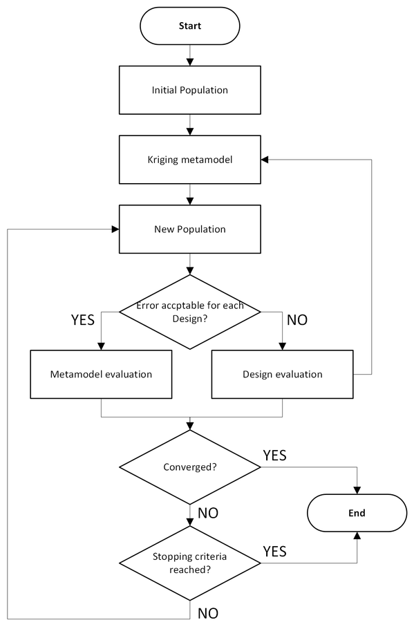
The AMO algorithm proceeds in the following steps:
Initial population of MOGA: the initial population of MOGA is used to construct the Kriging response surfaces.
Kriging generation: a Kriging response surface is created for each output, based on the first population and then enhanced during simulation with the addition of new design points.
MOGA: MOGA is run to generate the next population.
Evaluate the population: the population is evaluated on the Kriging response surface.
Error check: Kriging error predictor is checked for each design of the new population. If the error for a given design point is acceptable, the approximated value provided by Kriging is included in the next population to be run through MOGA (return to Step 3). If the error is not acceptable, the design point is promoted as new design point to evaluate an the real solver. The new design points are used to improve the Kriging response surface (return to Step 2) and are included in the next population to be run through MOGA (return to Step 3).
Convergence check: the optimization is validated for convergence. MOGA converges when the maximum allowable Pareto percentage has been reached. When this happens, the process is stopped. If the optimization is not converged, the process continues to the next step.
Stopping criteria: if the optimization has not converged, it is validated for fulfillment of the stopping criteria. When the maximum number of iterations has been reached, the process is stopped without having reached convergence. If the stopping criteria have not been met, the MOGA algorithm is run again (return to Step 3).
Conclusion: Steps 2 through 7 are repeated in sequence until the optimization has converged or the stopping criteria have been met. When either of these things occurs, the optimization concludes.
Limitations: AMO does not support discrete parameters. It is limited to continuous parameters, including those with manufacturable values (list of continuous values).
Available in: ModelCenter, optiSLang
The application of evolutionary algorithms for solving multi-objective optimization problems has been established over the past two decades. The parallel search for a set of Pareto optimal solutions is the major advantage of this method. The optiSLang implementation is based on the Strength Pareto Evolutionary Algorithm 2 (SPEA2) (Zitzler, Laumanns, and Thiele 2001) and is characterized by the following principles:
Elitism is applied by using an archive of non-dominated individuals.
Fitness assignment is based on the dominance criterion.
Preservation of population diversity is realized by density estimation.
The algorithm starts with the random or manual initialization of the first population of
size  followed by the evaluation of all individuals. For the first generation
  (number of parents) individuals are selected out of the population for
reproduction. After the evaluation of all newborns both archive individuals and offspring are
assigned new fitness values. The
(number of parents) individuals are selected out of the population for
reproduction. After the evaluation of all newborns both archive individuals and offspring are
assigned new fitness values. The  best solutions form the archive of the next generation. The optimization stops
if the maximum number of generations has been reached or the archive stagnated. In contrast to
the single-objective nature-inspired optimization methods, fitness assignment of the
multi-objective EA always regards the whole population, because the criterion is based on the
comparison of individuals. The fitness assignment method is a dominance-based ranking which
takes into account by how many individuals a solution is dominated and how many individuals a
solution dominates. To preserve the diversity of the Pareto frontier an additional criterion is
introduced to the fitness assignment procedure. The distance of an individual to its
best solutions form the archive of the next generation. The optimization stops
if the maximum number of generations has been reached or the archive stagnated. In contrast to
the single-objective nature-inspired optimization methods, fitness assignment of the
multi-objective EA always regards the whole population, because the criterion is based on the
comparison of individuals. The fitness assignment method is a dominance-based ranking which
takes into account by how many individuals a solution is dominated and how many individuals a
solution dominates. To preserve the diversity of the Pareto frontier an additional criterion is
introduced to the fitness assignment procedure. The distance of an individual to its  -th nearest neighbor serves as an estimator of density. The intention is to
prefer solutions in less crowded regions of the objective space such as boundary
solutions.
-th nearest neighbor serves as an estimator of density. The intention is to
prefer solutions in less crowded regions of the objective space such as boundary
solutions.
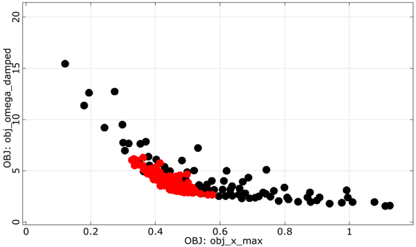
Figure 4.32: Pareto frontier for the damped oscillator (left) and Pareto optimal designs plotted in the design space (right) obtained by evolutionary algorithms
 |
 |
In Figure 4.32 the resulting Pareto frontier of the multi-objective evolutionary algorithm is shown for the damped oscillator example. The Pareto frontier shows a good agreement with the Pareto optimal designs from Figure 4.29. The Pareto frontier can now be used to judge about the importance of the different optimization goals and to choose a suitable optimal design. The efficiency of the multi-objective optimization methods can be dramatically improved especially for high-dimensional optimization problems by choosing a suitable start population instead of a pure random generation. Selected designs of a sensitivity analysis or previous optimization runs shall be used for this purpose.
References
Zitzler, E., M. Laumanns, and L. Thiele. 2001. "SPEA2: Improving the Strength Pareto Evolutionary Algorithm." 103. Computer Engineering; Networks Laboratory (TIK), Swiss Federal Institute of Technology (ETH) Zurich.
Available in: ModelCenter
Keywords— Natures-inspired, Evolutionary Algorithm
Darwin algorithm (see Section 4.2.5.2) can also be applied to multi-objective optimization problems. When more than one objectives are defined, Darwin will search for a series of best designs (Pareto set) using non-dominated design search.
Available in: ModelCenter, optiSLang
The Particle Swarm Optimization algorithm can also be applied to multi-objective optimization problems. As mentioned for single-objective PSO (see Section 4.2.5.6) optiSLang selects the fittest design as global leader. For the next iteration step the swarm will move in this direction. In multi-objective optimization the fitness evaluation is different from the single-objective approach.
Fitness assignment of the multi-objective PSO is similar to EA (Section 4.3.5.1).
Available in: LS-OPT, ModelCenter
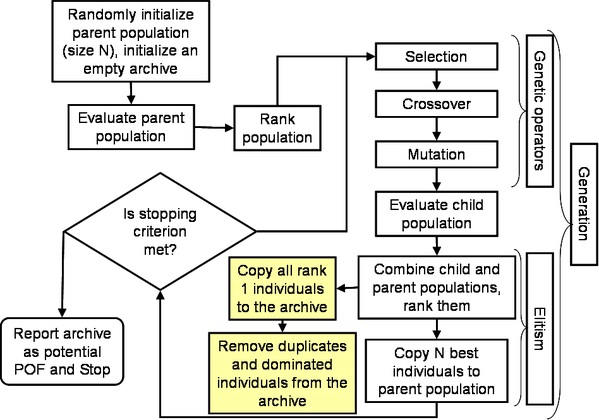
This algorithm was developed by Prof. Kalyanmoy Deb and his students in 2000 (Deb et al. 2002). This algorithm first tries to converge to the Pareto optimal front and then it spreads solutions to get diversity on the Pareto optimal front. Since this algorithm uses a finite population size, there may be a problem of Pareto drift. To avoid that problem, Goel et al.(Goel et al. 2007) proposed maintaining an external archive.
The implementation of this archived NSGA-II is shown in Figure 4.33, and described as follows:
Randomly initialize the parent population (size
 ). Initialize an empty archive.
 Evaluate the population i.e., compute constraints and objectives for each individual.
Rank the population using non-domination criteria. Also compute the crowding distance (this distance finds the relative closeness of a solution to other solutions in the function space and is used to differentiate between the solutions on same rank).
Employ genetic operators - selection, crossover & mutation - to create a child population.
Evaluate the child population.
Combine the parent and child populations, rank them, and compute the crowding distance.
Apply elitism (defined in a following section): Select best
 individuals from the combined population. These individuals constitute the
parent population in the next generation.
individuals from the combined population. These individuals constitute the
parent population in the next generation. Add all rank = 1 solutions to the archive.
Update the archive by removing all dominated and duplicate solutions.
If the termination criterion is not met, go to step 4. Otherwise, report the candidate Pareto optimal set in the archive.
Figure 4.33: Elitist non-dominated sorting genetic algorithm (NSGA-II). The shaded blocks are not the part of original NSGA-II but additions to avoid Pareto drift.
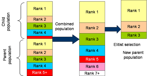
Elitism is applied to preserve the best individuals. The mechanism used by NSGA-II algorithm
for elitism is illustrated in Figure 4.34.
After combining the child and parent populations, there are 2 individuals. This combined pool of members is ranked using non-domination
criterion such that there are
individuals. This combined pool of members is ranked using non-domination
criterion such that there are  individuals with rank
  . The crowding distance of individuals with the same rank is computed. Steps in
selecting
. The crowding distance of individuals with the same rank is computed. Steps in
selecting  individuals are as follows:
Set
 , and number of empty slots
  .
. If
 ,
, Copy all individuals with rank "
 " to the new parent population.
 Reduce the number of empty slots by
 :
:  .
. Increment "
 ":
":  .
. Return to Step 2.
If
 ,0.
,0. Sort the individuals with rank "
 " in decreasing order of crowding distance.
 Select
 individuals.
 Stop.
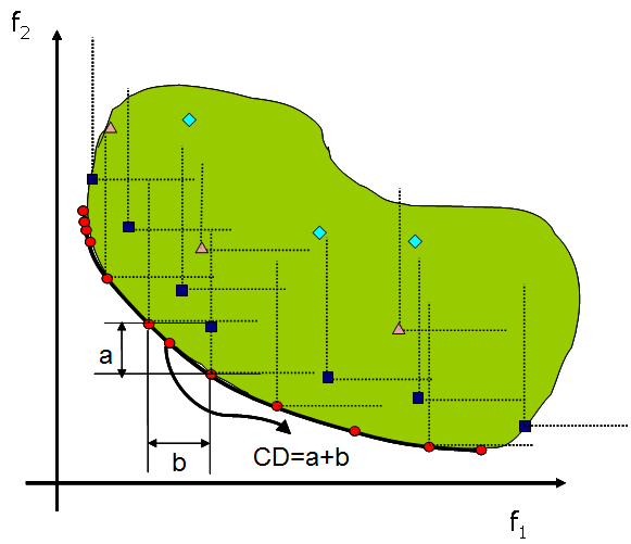
To preserve diversity on the Pareto optimal front, NSGA-II uses a crowding distance
operator. The individuals with same rank are sorted in ascending order of function values. The
crowding distance is the sum of distances between immediate neighbors, such that in Figure 4.35, the
crowding distance of selected individual is " ". The individuals with only one neighbor are assigned a very high crowding
distance. Note: It is important to scale all functions such that they are of the same order of
magnitude otherwise the diversity preserving mechanism would not work properly.
". The individuals with only one neighbor are assigned a very high crowding
distance. Note: It is important to scale all functions such that they are of the same order of
magnitude otherwise the diversity preserving mechanism would not work properly.
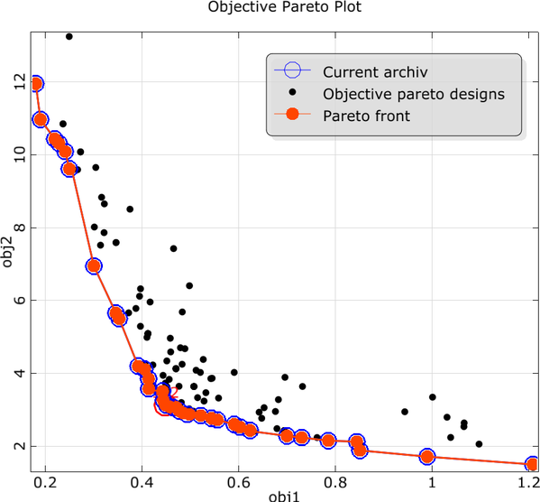
Figure 4.35: Illustration of non-domination criterion, Pareto optimal set, and Pareto optimal front.
NSGA II improved the original NSGA by adding following capabilities:
Faster sorting algorithm to compute Pareto set.
Elitist approach is used to preserve best designs from previous generations.
In multi-objective optimization, finding diverse designs is important. If a design is close to another design, a process called "sharing" is used to penalize such points. NSGA II uses more robust sharing technique that does not require control parameters.
References
Deb, Kalyanmoy, Amrit Pratap, Sameer Agarwal, and TAMT Meyarivan. 2002. "A Fast and Elitist Multiobjective Genetic Algorithm: NSGA-II." IEEE Transactions on Evolutionary Computation 6 (2): 182–97.
Goel, Tushar, Rajkumar Vaidyanathan, Raphael T Haftka, Wei Shyy, Nestor V Queipo, and Kevin Tucker. 2007. "Response Surface Approximation of Pareto Optimal Front in Multi-Objective Optimization." Computer Methods in Applied Mechanics and Engineering 196 (4-6): 879–93.
Available in: DesignXplorer
The Multi-Objective Genetic Algorithm (MOGA) is a hybrid variant of the popular NSGA-II (Non-dominated Sorted Genetic Algorithm-II) based on controlled elitism concepts. It supports all types of input parameters. The Pareto ranking scheme is done by a fast, non-dominated sorting method that is an order of magnitude faster than traditional Pareto ranking methods. The constraint handling uses the same non-dominance principle as the objectives. Therefore, penalty functions and Lagrange multipliers are not needed. This also ensures that the feasible solutions are always ranked higher than the infeasible solutions.
The first Pareto front solutions are archived in a separate sample set internally and are distinct from the evolving sample set. This ensures minimal disruption of Pareto front patterns already available from earlier iterations. The basic steps of the MOGA algorithm are as follows:
Initialize the population.
Evaluate the initial population members (calculate the values of the objective function(s) and constraints for each population member).
Loop until converged, or stopping criteria reached.
Perform crossover.
Perform mutation.
Evaluate the new population.
Assess the fitness of each member of the population so as to select members to be replaced in next step.
Replace population with members selected to continue in the next generation.
Apply niche pressure to the population to generate a more even and uniform sampling by encouraging differentiation along the Pareto frontier.
Test for convergence.
Available in: ModelCenter, optiSLang
Keywords— Hybrid optimization, Success factor
The One-Click Optimization (OCO) method is a hybrid and dynamic optimization approach. It efficiently combines direct (high-fidelity model) and MOP (low fidelity model) assisted search strategies. OCO is a general purpose optimizer that automatically and iteratively selects the most suitable optimization methods exposed by optiSLang.
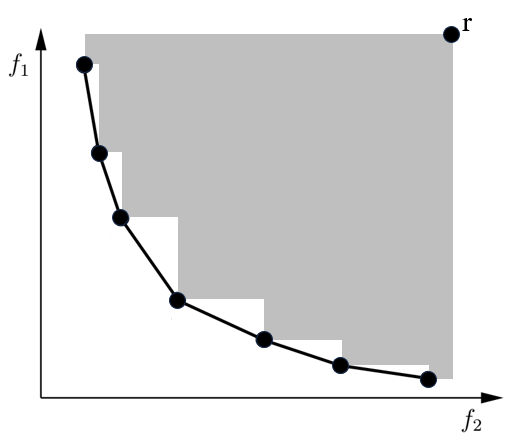
The main difference between the OCO approach for multi-objective optimization and the OCO approach for single-objective optimization (see Section 4.2.6.1) is the computation of the success factor. In multi-objective applications, the hypervolume indicator (see Figure 4.36) is an integral part of the success factor, used to evaluate the success of an optimization algorithm and rank optimization algorithms with a scalar metric.
This is the number of solutions of all nondominated solutions at any generation. Usually a higher number of nondominated points are achieved when convergence is good.
The spread of the front is calculated as the diagonal of the largest hypercube in the function space that encompassed all points. A large spread is desired to find diverse trade-off solutions. The spread measure is derived using the extreme solutions making it susceptible to the presence of a few isolated points that could artificially improve the spread metric. An equivalent criterion might be the volume of such a hypercube.
This complimentary criterion (to the spread metric) detects the presence of poorly distributed solutions by estimating how uniformly the points are distributed in the Pareto optimal set. This metric is defined as,
 | (4–40) |
where  is the crowding distance of the solution in the function or variable space.
The boundary points are assigned a crowding distance of twice the distance to the nearest
neighbor. A small value of the uniformity measure is desired to achieve a good distribution of
points.
is the crowding distance of the solution in the function or variable space.
The boundary points are assigned a crowding distance of twice the distance to the nearest
neighbor. A small value of the uniformity measure is desired to achieve a good distribution of
points.
This represents the range of individual objectives. A wide range represents more choices for the designer.
The hypervolume indicator was first proposed as a method for assessing multiobjective optimization algorithms (Zitzler and Thiele 1999). A dominated hypervolume metric tries to simultaneously estimate the convergence and spread characteristics by computing the union of the volume between the optimal solutions and a reference point. For practical purposes, the nadir point of all solutions is used as the reference point. While all the above metrics are obtained on a single set of solutions, the following performance metrics are obtained by comparing multiple sets of solutions. These metrics are helpful in determining the convergence.


References
Zitzler, Eckart, and Lothar Thiele. 1999. "Multiobjective Evolutionary Algorithms: A Comparative Case Study and the Strength Pareto Approach." IEEE Transactions on Evolutionary Computation 3 (4): 257–71.
This is the number of solutions that exist in both sets  and
and  . A large number of common points is indicative of the high quality of
solutions. The set of common solutions is represented as,
. A large number of common points is indicative of the high quality of
solutions. The set of common solutions is represented as,
 | (4–41) |
and  is the size of set
  . This is a particularly good metrics when a large generation interval is used.
This metrics denotes the number of nondominated solutions that were evolved during the current generation interval. The set of such solutions is represented as,
 | (4–42) |
A large number of new solutions relative to the total archive size indicates that the new solutions are still being evolved and hence convergence is not yet achieved.
This metrics denotes the number of nondominated solutions in the older archive  that were dominated by the solutions in the current archive
  . The set of dominated solutions is,
 | (4–43) |
A large number of new solutions relative to the total archive size indicates that the new solutions are still being evolved and hence convergence is not yet achieved.
This represents the fraction of archive  that has evolved up to the
  generation. This is computed as the ratio of the number of members in archive
 that are also present in the archive
  (non-dominated solutions) to the size of archive
  . Mathematically,
 | (4–44) |
This metric represents the proportion of potentially converged solutions in the
archive. In the early phase of a multi-objective evolutionary algorithm (MOEA) simulation, a
large fraction of the non-dominated solutions in the archive  would be dominated by the solutions in archive
  due to evolution, thus resulting in a small fraction of surviving solutions
i.e., small value of the consolidation ratio. However, significantly better solutions
evolve in the later phases such that a large proportion of solutions in the archive
due to evolution, thus resulting in a small fraction of surviving solutions
i.e., small value of the consolidation ratio. However, significantly better solutions
evolve in the later phases such that a large proportion of solutions in the archive
 remain non-dominated with respect to new solutions leading to a high
consolidation ratio. In the limiting case, the consolidation ratio approaches one.
remain non-dominated with respect to new solutions leading to a high
consolidation ratio. In the limiting case, the consolidation ratio approaches one.
This represents the fraction of archive  dominated by the new solutions in archive
  . This is computed as the ratio of the number of members in archive
  that are dominated by the solutions in archive
  (dominated solutions) to the size of archive
  . Mathematically,
 | (4–45) |
The archive  includes all non-dominated members of archive
  so no member of the archive
  is dominated. The improvement ratio quantifies the extent of improvement in
the quality of evolved solutions. This metric has a high value in the early phase of simulation
which gradually converges to zero when convergence is achieved.
is dominated. The improvement ratio quantifies the extent of improvement in
the quality of evolved solutions. This metric has a high value in the early phase of simulation
which gradually converges to zero when convergence is achieved.
More information about these performance metrics can be obtained from (Goel and Stander 2010).
References
Goel, Tushar, and Nielen Stander. 2010. "A Non-Dominance-Based Online Stopping Criterion for Multi-Objective Evolutionary Algorithms." International Journal for Numerical Methods in Engineering 84 (6): 661–84.