


Optimization can be defined as a procedure for achieving the best outcome of a given operation while satisfying certain restrictions. This objective has always been central to the design process, but is now assuming greater significance than ever because of the maturity of mathematical and computational tools available for design.
In single and multi-objective optimization the optimization task has to be defined by means of the objective functions:
 | (4–1) |
which can be implicit functions of the input variables
 and of scalar and non-scalar response values
 .
In optiSLang the user can define minimization and maximization
task with scalar objective functions, where the full calculator
functionality can be applied. For non-scalar response values such
as signal outputs, scalarization functions are available to derive
scalar measures for the definition of the objectives such as
integral values, deviation between two signals and many more.
.
In optiSLang the user can define minimization and maximization
task with scalar objective functions, where the full calculator
functionality can be applied. For non-scalar response values such
as signal outputs, scalarization functions are available to derive
scalar measures for the definition of the objectives such as
integral values, deviation between two signals and many more.
In unconstrained optimization problems only the bounds or values
of the design variables limit the optimization space. The
optimizer searches between these limits for the minimum value of
the objective function
 .
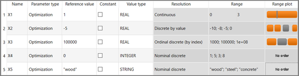
For maximization problems the sign of the user-defined objective
function is inverted in optiSLang to get a minimization task. The
design variables can be defined as continuous variables with a
lower and upper bound or as discrete variables which assume
several discrete values. In
Figure 4.1 the
definition of different optimization parameters types for
optiSLang is shown. The discrete parameters are distinguished as
discrete by value, which use the real data axis, ordinal discrete,
which use the ordered ordinal axis, and nominal discrete, which
may contain completely unordered states having real, integer or
string value types.
.
For maximization problems the sign of the user-defined objective
function is inverted in optiSLang to get a minimization task. The
design variables can be defined as continuous variables with a
lower and upper bound or as discrete variables which assume
several discrete values. In
Figure 4.1 the
definition of different optimization parameters types for
optiSLang is shown. The discrete parameters are distinguished as
discrete by value, which use the real data axis, ordinal discrete,
which use the ordered ordinal axis, and nominal discrete, which
may contain completely unordered states having real, integer or
string value types.
In engineering problems often additional restrictions have to be fulfilled by the optimal design. With help of equality and inequality constraints:

such restrictions can be formulated. The constraint functions can represent limitations depending only on the input variables but also depending on all available model responses and any mathematical combination of both.
Equality constraints are very difficult to treat. Therefore, it is not allowed to define equality constraints in optiSLang. However, equality constraints fulfilled with a given tolerance can be formulated easily as inequality constraints and in that way they can be handled by all optimization methods available in optiSLang. In order to get an optimal convergence of the optimizer and sufficiently accurate fulfillment of the constraint conditions, it is very useful to scale the objective and the constraint functions to be in a similar range. This can be realized e. g. by using the results of the design exploration.
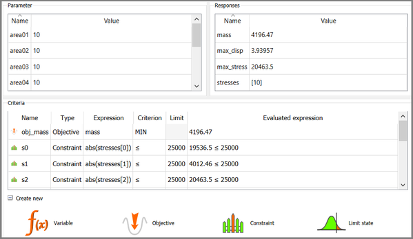
In Figure 4.2 the typical setup of the optimization criteria, objectives functions and constraints, is shown. The objective functions can be defined as maximization or minimization goals, whereas the constraint function contain a left and a right functional term within a greater equal or less equal definition.
Table 4.1 describes the properties and a suggested application for each optimizer introduced in this documentation.
Table 4.1: Available optimization algorithms with application for single and multi-objective optimization and possible discrete inputs variables
| Optimizer | Objectives | Discrete inputs | |||
| Single | Multi | by value | ordinal | nominal | |
| Hybrid methods | |||||
| One Click Optimization | yes | yes | yes | yes | no |
| Gradient-based methods | |||||
| Non-Linear Programming (NLPQLP) | yes | no | no | no | no |
| Mixed Integer SQP | yes | no | yes | yes | no |
| Leapfrog Optimization (LFOPC) | yes | no | (yes) | (yes) | no |
| DAKOTA Coliny Solis-Wets | yes | no | no | no | no |
| DAKOTA Coliny CONMIN | yes | no | no | no | no |
| DAKOTA Coliny FDN | yes | no | no | no | no |
| DAKOTA Coliny Quasi Newton (QN) | yes | no | no | no | no |
| DAKOTA Coliny PR | yes | no | no | no | no |
| Pattern search methods | |||||
| Downhill simplex | yes | no | (yes) | (yes) | no |
| Hooke-Jeevs Pattern Search | yes | no | no | no | no |
| DAKOTA OPT++ Parallel Direct Search | yes | no | no | no | no |
| DAKOTA APPS | yes | no | no | no | no |
| DAKOTA Coliny DIRECT | yes | no | no | no | no |
| DAKOTA Coliny Pattern Search | yes | no | no | no | no |
| Response surface based methods | |||||
| Adaptive Response Surface Method (ARSM) | yes | no | yes | yes | no |
| Adaptive MOP (AMOP) | yes | yes | yes | yes | no |
| Adaptive Single-Objective (ASO) | yes | no | yes | yes | no |
| Adaptive Multi-Objective (AMO) | no | yes | yes | yes | no |
| Efficient Global Optimization (UP-EGO) | yes | no | yes | yes | no |
| Bayesian Optimization (PI-BO) | yes | no | yes | yes | (yes) |
| Nature-inspired methods | |||||
| Evolutionary Algorithm (EA) | yes | yes | yes | yes | yes |
| Darwin algorithm | yes | yes | yes | yes | yes |
| DAKOTA Coliny Evolutionary Algorithm | yes | no | yes | yes | yes |
| EVOLVE | yes | no | yes | yes | yes |
| Covariance Matrix Adaptation (CMA) | yes | no | yes | yes | (yes) |
| Particle Swarm Optimization (PSO) | yes | yes | yes | yes | (yes) |
| Stochastic Design Improvement (SDI) | yes | no | yes | yes | yes |
| Adaptive Simulated Annealing | yes | no | yes | yes | (yes) |
| Differential Evolution | yes | no | yes | yes | (yes) |