


An FE body represents the motion of a deformable body, with degrees of freedom directly proportional to either the number of nodes within the body or the modes of vibration it supports. This concept is crucial in simulations where the deformation or dynamic response of bodies under various loads and boundary conditions is of interest.
Deformable bodies in Motion are primarily categorized into two types: Nodal FE Bodies and Modal FE Bodies. Understanding the distinctions and applications of each type enables more accurate and efficient simulation of real-world phenomena.
Incorporating FE bodies into simulations allows for the accurate modeling of parts where deformation impacts the overall system behavior, such as in vibration analysis or when assessing structural integrity under dynamic loads. By capturing the transmission of vibrations and the deformation characteristics of these components, engineers can predict the performance and identify potential failure modes more effectively.
The Nodal FE Body approach models deformation by utilizing the finite element method (FEM), where the mesh's nodes determine the body's degrees of freedom. This method is particularly effective for detailed local analysis, where stresses and strains need to be accurately captured at specific points. Nodal FE Bodies are generated from meshes developed in Ansys Mesh or other compatible meshing tools.
The Degrees of Freedom (DOFs) of a Nodal FE Body are determined by the number of nodes and the types of elements used, such as beam, shell, or solid elements. Nodes associated with beam and shell elements have six DOFs (three translational and three rotational) while nodes in solid elements possess three translational DOFs. Additionally, to represent the overall behavior of the body, six DOFs (three translational and three rotational) are also attributed to the flexible body reference frame, which is also referred to as a moving reference frame.
Nodal coordinates define the displacement and rotation of nodes in a finite element model, representing the deformation and movement of elements under various conditions. The nodal coordinates represent the deformation in three translational DOFs for solid elements or six DOFs for beam or shell elements. The rotational DOFs can represent by using the Euler angles. Equation of motion of this body is formulated with the inertia force and elastic force from the finite elements.
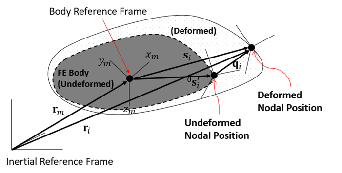
The initial position of the body reference frame can be located either at the mass center or elsewhere on the body and its orientation is assumed to be the identity matrix. The position and orientation of the node can be represented by the following equations:
 | (3–15) |
 | (3–16) |
where:
 = position of the node = position of the node |
 = orientation of the node = orientation of the node |
 = position of the moving reference frame = position of the moving reference frame |
 = orientation of the moving reference frame = orientation of the moving reference frame |
 = translational deformations of the nodal
coordinates = translational deformations of the nodal
coordinates |
 = rotational deformations of the nodal
coordinates = rotational deformations of the nodal
coordinates |
 = relative orientation of the node with respect to the
moving reference frame. is a
function of . = relative orientation of the node with respect to the
moving reference frame. is a
function of . |
 = relative displacement from the moving reference
frame to the node with respect to the moving reference frame at the
initial time. = relative displacement from the moving reference
frame to the node with respect to the moving reference frame at the
initial time. |
In the nodal FE body, the generalized coordinates are rm, θm, ri, and θi. Here, θm represents the Euler angles obtained from the orientation Am of the moving reference frame.
If the orientation Am of the flexible body represents the global rotation of the flexible body, this setup offers improved analytical performance and solution accuracy in problems involving rotations of the flexible body. However, if the moving reference frame undergoes significant deformations or oscillations, even small changes in the orientation of the moving reference frame can affect the nodal displacements across all nodes, potentially degrading convergence. The solver therefore adopts the following strategy based on the analysis settings:
If the High-speed Rotation option is activated or if the Super solver type is utilized, Am will represent the orientation of the flexible body.
Otherwise, Amwill be treated as an identity matrix, and the displacements at each node will reflect rotations.
The position of the center of mass of the FE body can be calculated as follows:
 | (3–17) |
where:
 = the total number of nodes in the nodal FE
body = the total number of nodes in the nodal FE
body |
 = the mass of the nodes belonging to the nodal FE
body = the mass of the nodes belonging to the nodal FE
body |
 = the total mass of the nodal FE body, as calculated
below: = the total mass of the nodal FE body, as calculated
below: |
 | (3–18) |
The mass moment of inertia in the inertia reference frame can be calculated from the following equation:
 | (3–19) |
where:
 = relative displacement from the moving reference
frame to the node = relative displacement from the moving reference
frame to the node |
 = mass moment of inertia of the node with respect to
the coordinate system on the node = mass moment of inertia of the node with respect to
the coordinate system on the node |
The nodal mass and mass moment of inertia can be calculated by averaging the masses of adjacent finite elements. For the solid elements, the nodal mass moment of inertia is zero.
The velocities of the node are derived from the time derivatives of the node's position and orientation, and can be expressed as follows:
 | (3–20) |
 | (3–21) |
 | (3–22) |
where:
 = translational velocity of the node = translational velocity of the node |
 = angular velocity of the node = angular velocity of the node |
 = angular velocity of the node with respect to moving
reference frame = angular velocity of the node with respect to moving
reference frame |
 = translational velocity of the moving reference
frame = translational velocity of the moving reference
frame |
 = angular velocity of the moving reference
frame = angular velocity of the moving reference
frame |
 = time derivative of the translational deformations of
the nodal coordinates = time derivative of the translational deformations of
the nodal coordinates |
 = time derivative of the rotational deformations of
the nodal coordinates = time derivative of the rotational deformations of
the nodal coordinates |
 = time derivative of the relative orientation of the
node with respect to the moving reference frame. = time derivative of the relative orientation of the
node with respect to the moving reference frame. |
 = angular velocity transformation matrix for the Euler
angles = angular velocity transformation matrix for the Euler
angles |
The accelerations of the node are defined as follows.
 | (3–23) |
 | (3–24) |
 | (3–25) |
where:
 = translational acceleration of the node = translational acceleration of the node |
 = angular acceleration of the node = angular acceleration of the node |
 = angular acceleration of the node with respect to
moving reference frame = angular acceleration of the node with respect to
moving reference frame |
 = translational acceleration of the moving reference
frame = translational acceleration of the moving reference
frame |
 = angular acceleration of the moving reference
frame = angular acceleration of the moving reference
frame |
 = second time derivative of the translational
deformations of the nodal coordinates = second time derivative of the translational
deformations of the nodal coordinates |
 = second time derivative of the rotational
deformations of the nodal coordinates = second time derivative of the rotational
deformations of the nodal coordinates |
 = time derivative of the angular velocity
transformation matrix for the Euler angles = time derivative of the angular velocity
transformation matrix for the Euler angles |
The equation of motion for the node can be represented with the inertia force and elastic force as follows:
 | (3–26) |
 | (3–27) |
where:
 = force applied on the node = force applied on the node |
 = torque applied on the node with respect to the
coordinate system on the node = torque applied on the node with respect to the
coordinate system on the node |
 = elastic force by the element applied on the
node = elastic force by the element applied on the
node |
 = elastic torque by the element applied on the
node = elastic torque by the element applied on the
node |
The force and torque may originate from various entities such as joints, forces, contacts, and FE elements. For more information on calculating element forces, see Elastic Forces.
The force and torque on the node are calculated from the elementary forces as follows:
 | (3–28) |
where  and
and  are the element stiffness matrix for the node and the damping
ratio, respectively.
are the element stiffness matrix for the node and the damping
ratio, respectively.  and
and  are the deformation of the node and its time
derivative.
are the deformation of the node and its time
derivative.
For the general case, the element stiffness matrix can be calculated using the following equation:
 | (3–29) |
where  and
and  are the partial derivative of the shape function for the
finite element and the strain-stress relationship which is defined from the
material properties.
are the partial derivative of the shape function for the
finite element and the strain-stress relationship which is defined from the
material properties.
The nodal strain and stress can be calculated using the following equations:
 | (3–30) |
 | (3–31) |
where  is the nodal displacement.
This section explains how the Motion solver behaves with additional masses defined at specific locations, patches, edges, or individual nodes on the Nodal FE body. Ansys Motion supports three types of additional mass: Point Mass, Direct Attachment, and Distributed Mass.
A Point Mass defines a concentrated mass at a specific location on the Nodal FE Body. When a point mass is defined for a remote point or RBE (rigid body element), the mass of the interface node is set to the mass value set by the user.
A Direct Attachment allows mass to be added directly to the specified node. The mass added by the user is added to the selected node.
A Distributed Mass adds mass for nodes that belong to a patchset or edgeset by the effective area or length of each node.
The effective area and effective length of the ith node are:
 | (3–32) |
 | (3–33) |
The mass added to the ith node is:
 | (3–34) |
where:
 = mass per unit area (user input) = mass per unit area (user input) |
 = mass per unit length (user input) = mass per unit length (user input) |
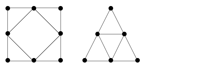
Limitation of Distributed Mass for High-order Elements
Patches belonging to high-order elements are divided into triangular patches with three nodes and quadrilateral patches with four nodes before being input into the solver. The effective area of a node is also calculated from these divided patches, so be cautious as the proportion of mass added to the mid-node may increase or the mass distribution may become non-uniform.
Position, velocities, acceleration, deformation, strain and stress of nodes and elements which belong to an FE body are output as described in FE Body Output in the Motion Preprocessor User Guide.
In Motion, a Modal FE Body represents a flexible body with a reduced degree of freedom of modal coordinates. This type of body is modeled by importing an FE data file and a modal data file in a mesh. The degree of freedom of the body is determined by the number of modes.
A Modal FE Body is defined through the technique of modal synthesis, which simplifies the representation of deformation in a system by utilizing a select number of modes. These modes are obtained through a process known as modal analysis, specifically through eigenvalue analysis in Motion, Ansys Modal or other FEA software. Each mode is distinguished by its unique deformation pattern and corresponding frequency, playing a crucial role in defining the overall dynamic behavior of the system. By focusing on these essential modes, modal synthesis generally aims to significantly reduce the required computational resources while accurately capturing the system's critical dynamic phenomena.
Modal synthesis is a method of strategically selecting and combining these modes to construct a comprehensive model of the system's dynamic response. This approach is particularly useful when gaining detailed insight into the global dynamic behavior is more important than understanding local stress distribution. The modal synthesis method is highly effective in the field of Noise, Vibration, and Harshness (NVH) analysis, accurately depicting the system's resonance characteristics, which are fundamental for evaluating and improving performance. The modal synthesis method provides the best solutions within the linear range and is not a good method when load conditions frequently change, such as with large deformations or contact problems. While the modal FE body may have limitations in depicting local deformations or stresses compared to the nodal FE body, it has the advantage of providing better analysis performance with fewer degrees of freedom. Using this method allows engineers to delicately balance the need for computational efficiency and accurate dynamic behavior analysis. However, it is important to carefully evaluate the results to ensure they are a good approximation of accurate outcomes.
The degrees of freedom for a Modal FE Body correspond to the number of modes. Additionally, to represent the overall behavior of the body, six degrees of freedom (three translational and three rotational) are also attributed to the flexible body reference frame.
A modal FE body has a moving reference frame to represent the rigid motion in six DOFs and modal coordinates to represent the deformation. The nodal equation of motion of a modal FE body is exactly the same as those of a nodal FE body, which is formulated with the inertia force and elastic force.
The main difference between a modal FE body and a nodal FE body is how to represent the deformation of each node. For a nodal FE body, the deformation of the nodal coordinates qi and θi become the generalized coordinates. On the other hand, for a modal FE body, the modal coordinate is used as the generalized coordinate. This method decreases the degree of freedom by projecting the nodal displacements into the modal space and reformulating the equations of motion in the modal space.
The translational and rotational displacements of a node and their time derivatives are calculated with the modal coordinate and mode shape as follows:
 | (3–35) |
 | (3–36) |
 | (3–37) |
where:
 = mode shape of the
ith node in three or six
by the number of modes = mode shape of the
ith node in three or six
by the number of modes |
 = modal coordinates = modal coordinates |
 = time derivative of the modal coordinates = time derivative of the modal coordinates |
 = second time derivative of the modal
coordinates = second time derivative of the modal
coordinates |
From the nodal deformation and its time derivative obtained from the above equations, the position, velocity, and acceleration of the node are obtained in the same way as for a nodal FE body.
The nodal equation of motion, which is calculated using the inertia force and elastic force, can be projected into the modal space as follows:
 | (3–38) |
 | (3–39) |
where:
 = translational mode shape of
ith node = translational mode shape of
ith node |
 = rotational mode shape of ith
node = rotational mode shape of ith
node |
 = force applied on the interface node = force applied on the interface node |
 = torque applied on the interface node with respect to the
coordinate system on the interface node = torque applied on the interface node with respect to the
coordinate system on the interface node |
 = elastic force applied on the interface node = elastic force applied on the interface node |
 = elastic torque applied on the interface node = elastic torque applied on the interface node |
The force and torque may be generated from any entity, such as a joint or force.
The elastic force and torque in the modal space can be written as follows:
 | (3–40) |
where:
 = eigenvalue of the modal FE body = eigenvalue of the modal FE body |
 = damping coefficient which is proportional to the
eigenvalue = damping coefficient which is proportional to the
eigenvalue |
The nodal strain and stress can be calculated as for a nodal FE body.
Invariant variables of a modal FE body denote terms that are constant within the generalized forces, also known as residuals, derived from the motion equations of the modal FE body. These variables, which include mass, relative coordinates, and mode shape vectors, maintain their values regardless of changes in the body reference frame or modal coordinates. Due to the characteristics of invariant variables, there is a reduction in computational demand during complex analyses, and the physical properties of the system are maintained consistently, which is essential for the precise modeling and optimization of dynamic systems.
The position of the node in the modal body can be represented as follows:
 | (3–41) |
The translational motion equation of the node in the modal body can be expressed using the virtual work theory as follows:
 | (3–42) |
where:
 = virtual rotation of the body reference frame. = virtual rotation of the body reference frame.  |
From the above equation, the generalized forces Q for generalized coordinates  ,
,  and
and  can be expressed as follows.
 | (3–43) |
where:
 | (3–44) |
Upon substituting equation Equation 3–43 into Equation 3–44 and simplifying, the expression becomes as follows:
 | (3–45) |
In the above equation, ζ1 to ζ8 are invariant variables and are as follows:
 | (3–46) |
 | (3–47) |
 | (3–48) |
 | (3–49) |
 | (3–50) |
 | (3–51) |
 | (3–52) |
 | (3–53) |
Ansys Motion calculates invariant variables during Body Eigenvalue Analysis and stores them in a .dfmf file for reuse in subsequent analyses. If body eigenvalue analysis is conducted using other FEA software, this calculation is performed during the importation of modal data.
Modal damping describes the damping characteristics of individual vibration modes. It quantifies energy dissipation for each mode using damping coefficients, indicating how quickly vibrations decay. The damping coefficient in Equation 3–40 is calculated from the stiffness proportional damping ratio and eigenvalue:
 | (3–54) |
where:
 = stiffness proportional damping ratio for each mode,
given by = stiffness proportional damping ratio for each mode,
given by  |
The stiffness proportional damping ratio β is related to the damping ratio ζ and the natural frequency ωn of the system. The damping ratio ζ is a measure of how oscillations in a system decay after a disturbance, and it is defined as the ratio of the actual damping to the critical damping.
The stiffness proportional damping ratio for ith mode is:
 | (3–55) |
where:
 = damping ratio of ith
mode = damping ratio of ith
mode |
 = natural frequency of ith mode
in radians per second = natural frequency of ith mode
in radians per second |
 = natural frequency of ith mode
in Hz = natural frequency of ith mode
in Hz |
In this relationship, β indicates how the damping coefficient c is proportional to the stiffness of the system through the eigenvalue λ. By adjusting β, you can control the amount of damping in the system, directly influencing the system's dynamic response.
The output parameters for a Modal FE body are described in Modal FE Body Output in the Motion Preprocessor User Guide.