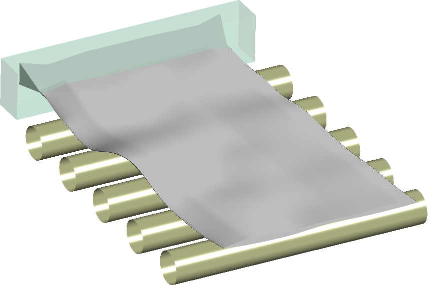
Consider the extrusion flow illustrated in Figure 3.256: Illustrative Simulation of the Extrusion of a Rubber Tire Tread (Grey) Out of a Part of a Die (Green Transparent) Assisted by a Roller Conveyor (Brown). From left to right along the flow direction, you can observe the solid die with part of the die lips, the extrudate undergoing visible deformations due to velocity rearrangement at the die exit and the effects of gravity, and finally, the extrudate being guided by a roller conveyor. By qualitatively examining the flow, you can uncover various physical phenomena and use this opportunity to introduce the symbols used later in this chapter.

Firstly, consider the flow of a highly viscous material, such as rubber. This involves calculating the velocity and stress fields, denoted as νand , respectively, in the fluid region. An important component of the stress field is the pressure , which, in polymer and rubber processing, can reach values as high as 500 bars or more. This pressure, in turn, is applied to the solid die, causing deformation and possibly requiring the calculation of elastic stresses and deformations in the solid die.

Additionally, the high viscosity of the fluid results in viscous heating, especially along the interface with the die, and naturally leads to changes in temperature and heat transfer. Upon exiting the die, the extrudate exchanges heat with the surrounding air and gradually cools down.

Figure 3.256: Illustrative Simulation of the Extrusion of a Rubber Tire Tread (Grey) Out of a Part of a Die (Green Transparent) Assisted by a Roller Conveyor (Brown)

As can be seen from this relatively standard application, a wide range of physics can be involved. However, in many similar situations, engineering common sense often suggests assumptions and simplifications, guiding which aspects of the physics are relevant and need to be simulated.

In most material processing cases, the fluid in motion (for example, polymer, rubber, or glass) is assumed to be incompressible. Under this assumption, the momentum and mass conservation equations governing the velocity and pressure are given as follows:

(3–191)

and

(3–192)

In the equations above, stands for the fluid density, while and represents the gravity (volume) force and the additional stress contribution of the fluid to the momentum balance, respectively. As shown, you have two equations for three unknowns , and . An additional equation is needed: a constitutive equation that describes the material response to a given kinematics. An entire section is dedicated to the several constitutive equations. To simplify the discussion, the simplest constitutive law is introduced: that of a constant-viscosity Newtonian fluid. For the Newtonian fluid, the extra-stress tensor is given by:

(3–193)

In Equation 3–193,   is the shear viscosity of the fluid, while   is the rate-of-deformation tensor given as the symmetric part of the velocity gradient tensor, for example:

(3–194)

The algebraic character of Equation 3–193 allows a direct substitution in Equation 3–191, which then becomes:

(3–195)

By invoking the incompressibility Equation 3–192, Equation 3–195 can formally be rewritten as:

(3–196)

In the absence of inertia terms and volume force, Equation 3–196 reduces to a diffusion equation for the velocity, which has to be solved together with the mass conservation Equation 3–192.

Even in the simplest case of a constant-viscosity Newtonian fluid, the fluid motion is governed by differential equations: hence boundary conditions are required, while sometimes initial conditions are also needed. In simple words, such boundary and initial conditions express the relationship of the calculation domain with the surrounding world and with past events, respectively.

In the context of a fluid flow, boundary conditions can be of various type. If you consider the extrusion flow illustrated in Figure 3.256: Illustrative Simulation of the Extrusion of a Rubber Tire Tread (Grey) Out of a Part of a Die (Green Transparent) Assisted by a Roller Conveyor (Brown), you already identified at least four different boundary conditions, namely an inlet, a wall, a free surface and an exit. These will be briefly reviewed, providing an opportunity to complete the present list.

The material enters the calculation domain at the inlet: a normal force or normal velocity distribution is imposed, which is combined with a vanishing tangential force or velocity. The easiest way of imposing a velocity distribution consists of specifying an inlet mass or volume flow rate.

Along a solid wall, vanishing velocity or stick condition is often imposed. However, in some circumstances the wall can be moving, while slipping at the wall can be encountered. In the present context, slipping conditions express a relationship between the tangential velocity and the tangential force in combination with a vanishing normal velocity. As such it is not a fluid property, instead, it is a fluid-solid interface property. The several slipping laws will be described in a subsequent section.

A free surface is a slightly more sophisticated boundary condition. In its simplest form, it involves vanishing forces in all directions with the additional requirement that the normal velocity be vanishing. It can be expressed by:

(3–197)

and

(3–198)

where is the geometric vector perpendicular to the free surface. In other words, you have more conditions than available degrees of freedom. In order to circumvent this, the boundary is allowed to deform in order to simultaneously satisfy the several requirements. Since the free surface condition is accompanied by the deformation of the boundary, the flow geometry itself is allowed to deform in the Eulerian sense.

For a transient flow, the free surface condition is extended by allowing a deformation of the boundary along the normal direction in the Lagrangian sense:

(3–199)

or along all directions when a Lagrangian representation is considered:

(3–200)

In the simplest model for the free surface given by Equation 3–197 and Equation 3–198, a stress-free boundary is assumed. However, additional inputs can be added. The first is the surface tension which depends on the curvature, and which then requires specifying a surface tension coefficient. For most applications involving polymer and rubber materials, surface tension is often negligible. An external pressure or vacuum can also be added: this is typically the case in applications like blow moulding and thermoforming, where such pressure is invoked for shaping an object. In such processes, the free surface will soon or later enter in contact with a fixed or moving mould: such a contact is also an external input to the free surface condition. Eventually, in steady extrusion processes, the boundary of the extrudate can also enter in contact with a guiding device, such as a roller conveyor as illustrated in Figure 3.256: Illustrative Simulation of the Extrusion of a Rubber Tire Tread (Grey) Out of a Part of a Die (Green Transparent) Assisted by a Roller Conveyor (Brown)

Boundary conditions, such as combinations of normal and tangential velocity or force, are also permitted. A particular case of such combination is the symmetry boundary condition consisting of a vanishing normal velocity and vanishing tangential force.

Next to the polymer flow, the extrusion process suggested in Figure 3.256: Illustrative Simulation of the Extrusion of a Rubber Tire Tread (Grey) Out of a Part of a Die (Green Transparent) Assisted by a Roller Conveyor (Brown) involves a die, for example, a solid body. Since polymer or rubber extrusion flows involve large pressures, it is sometimes instructive to examine the elastic behaviour of the die under high pressure applied at the interface. In the Polyflow software, it is considered that the assumptions of linear elasticity are satisfied under normal process conditions. However, it is sometimes relevant or instructive to evaluate the stress field in the die as well as the elastic displacement .

For a solid elastic body, the momentum equation is given by:

(3–201)

where stands for the elastic stress tensor. In view of the small size and the high elastic stiffness of the equipments, the acceleration term is usually neglected as is often the case for structure analysis in the present context. For solving Equation 3–201, consider the linear elasticity constitutive law given by:

(3–202)

In Equation 3–202, , and are respectively the Young modulus, the Poisson coefficient and the lineic thermal dilatation coefficient, while is the elastic strain tensor given as the symmetric part of the gradient of displacement. Eventually is the unit tensor.

When inserting the linear elasticity Equation 3–202 in the momentum equation (Equation 3–201), it is possible to obtain a second-order differential equation for the displacement . This equation requires boundary conditions on all sides of the calculation domain, which can be given is terms of assigned displacement or forces. Typically, boundary conditions can be vanishing displacements, vanishing normal displacement, vanishing forces, or external force imposed. This latter boundary condition is useful when performing a calculation involving a so-called fluid-structure interaction.

For a laminar flow, therefore at moderate velocity, as typically encountered in material processing, the energy equation can be written as follows:

(3–203)

In this equation, and are the heat capacity per unit volume and the thermal conductivity, respectively, these parameters can be temperature dependent and respectively affect the convection and the diffusion in the energy balance. The last two terms and of Equation 3–203 stand respectively for an external heat source and the viscous heating. Considering the high viscosity of polymers and rubbers, viscous heating may contribute to a visible temperature increase. On the contrary, kinetic and potential energy are negligible for laminar flows as encountered in industrial shaping processes.

For a solid body, Equation 3–203 still applies, however the transport term possibly involves an assigned velocity, while the viscous heating term is obviously discarded.

As can be seen, the temperature is governed by a second order differential equation, the advection-diffusion Equation 3–203. Therefore, as for the momentum equation, boundary conditions are required, while sometimes initial conditions are also needed. As previously formulated, such boundary and initial conditions express the relationship of the calculation domain with the surrounding world and with past events, respectively.

For the energy equation, boundary conditions are usually expressed in terms of imposed temperature or heat flux. In particular, a heat flux can be a constant quantity, a convective heat flux, or a radiative heat flux. Also, in a combined calculation involving a polymer flow and a die, as suggested in Figure 3.256: Illustrative Simulation of the Extrusion of a Rubber Tire Tread (Grey) Out of a Part of a Die (Green Transparent) Assisted by a Roller Conveyor (Brown), conjugated heat transfer is applied at the interface between the fluid and solid regions

Coming back to Equation 3–193 of the Newtonian fluid and for the sake of facility while introducing the flow governing equations, it is assumed that the viscosity parameter is constant. However, experimental data indicate that the shear viscosity usually decreases when the shear rate increases. A decay be several orders of magnitude is not exceptional. This phenomenon is known as shear-thinning. Therefore, for applications where shear stresses play a dominant role, it is a good idea to generalise Equation 3–193 and introduce a dependence of the shear viscosity with respect to the local shear rate .

If you consider the flow between two parallel plates with an inner-distance and a relative velocity , you can define the shear rate as:

(3–204)

Such a simple definition cannot be applied for a general 3D flow. Instead, make use of the so-called invariants of the rate-of-deformation tensor. The first invariant vanishes in view of the incompressibility, while the third invariant vanishes in a simple shear flow. Therefore, define the local shear rate based on the second invariant of as follows:

(3–205)

By doing so, you recover the result of Equation 3–204 in a simple shear flow.

Describing a shear-thinning behaviour is a matter of algebra. However physical aspects have to be taken into account. The scientific literature reports several laws able to mimic a shear-thinning behaviour, and most of them are available in the Polyflow software.

 

3.13.3.1.1. Power Law

The simplest shear-thinning viscosity law is the powerlaw written as

(3–206)

where is the consistency factor and is the power index of the shear viscosity. The quantity is introduced for enabling an easy conversion of units and can be set to 1. It is important to note however that both and cannot be selected independently. On a log-log scale, this law is represented as a straight line with a decreasing slope.

 

3.13.3.1.2. Bird-Carreau Law

With the Bird-Carreau law, you bound the shear viscosity for low shear rates, while viscosity plateau is introduced for high shear rates. The law is written as

(3–207)

In this context, the quantities and stand for the zero shear-rate and infinite shear-rate viscosities, respectively, while indicates the slope of the shear-thinning curve. Eventually, is the reciprocal of the cut-off shear rate or the shear rate which marks the location of the transition between the Newtonian plateau and the shear-thinning region.

 

3.13.3.1.3. Carreau-Yasuda Law

The Carreau-Yasuda law can be viewed as a generalization of Equation 3–207, and is written as:

(3–208)

In this case, the newly introduced parameter is an index which controls the transition from the Newtonian plateau to the shear thinning region. In particular a small value of a leads to a smooth transition.

 

3.13.3.1.4. Bingham Law

Some fluid materials are characterised by a yield stress and is typically the case for materials like concrete, mud, dough and toothpaste. In this first approximation, yield stress behaviour can be described by means of the Bingham law given by:

(3–209)

is the yield stress and is the critical shear rate beyond which a viscous behaviour is observed. Below this critical shear rate, the model is adjusted to guarantee the required continuity of the viscosity curve.

 

3.13.3.1.5. Modified Bingham Law

It is at times useful to have an analytical expression for describing yield behaviour. The Modified Bingham law, as an approximation of Equation 3–209, is given by

(3–210)

You should note that both Equation 3–209 and Equation 3–210 do exhibit nearly identical viscosity behaviour for shear rates beyond .

 

3.13.3.1.6. Herschel-Bulkley Law

Some yield stress fluid materials also exhibit a visible shear thinning at high shear rates. This behaviour can be described with the Herschel-Bulkley law given by

(3–211)

As for the Bingham law, is the yield stress and is the critical shear rate beyond which a viscous behaviour is observed. Below this critical shear rate, the model is adjusted to guarantee the required continuity of the viscosity curve.

 

3.13.3.1.7. Modified Herschel-Bulkley Law

It can be useful to have an analytical expression for describing yield behaviour combined with shear thinning at high shear rates. The Modified Herschel-Bulkley law, as an approximation of Equation 3–211, is given by:

(3–212)

You should note that both Equation 3–211 and Equation 3–212 do exhibit nearly identical viscosity behaviour for shear rates Equation 3–211 beyond Equation 3–212.

 

3.13.3.1.8. Cross Law

Back to more classical shear-thinning fluid models, it is important to mention the Cross law given by:

(3–213)

The parameter is the Cross law index. For large shear rates, it can be interpreted to as the quantity of the Bird-Carreau law. This law is characterised by a stretched transition between a plateau at low shear rates and the shear-thinning region at high shear rates.

 

3.13.3.1.9. Modified Cross Law

Finally, it is important to mention the Modified Cross law, which is expressed by:

(3–214)

The meaning of the parameters is identical as for Equation 3–213 However, the transition from the plateau at low shear rates to the shear thinning region is sharper than with the Cross law.

For thermal flows, the temperature dependence of the viscosity must be taken into account along with the shear-rate dependence. This is usually done by separating both dependences. Therefore, the viscosity law can be factorized as

(3–215)

or as

(3–216)

In Equation 3–215 and Equation 3–216, the function , corresponding to the shift factor, denotes the dependence with respect to the temperature while is the shear rate dependence law at a selected reference temperature , for example, when , and can be viewed as the master curve. Equation 3–215 is used when the temperature dependence of the viscosity involves only a vertical shift of the viscosity curve, while Equation 3–216 is considered when the temperature dependence of the viscosity simultaneously involves a vertical and a horizontal shift of the viscosity curve when the temperature changes.

 

3.13.3.2.1. Arrhenius Law

In the context of generalized Newtonian fluid flows, four laws are available for describing the temperature dependence of the viscosity . First, you have the Arrhenius law expressed by:

(3–217)

The quantity is the ratio of the activation energy to the thermodynamic constant while is the reference temperature for which , and which corresponds to the temperature of the master curve for the shear rate dependence of the viscosity. This dependence is typical for polymers and rubber materials.

 

3.13.3.2.2. Approximate Arrhenius Law

When the temperature range is narrow, you can invoke the approximate Arrhenius law instead of using Equation 3–217, and which consists of considering the first term of the Taylor series applied to the argument of the exponential. This provides:

(3–218)

In this case, the parameters have the same meaning as in Equation 3–217.

 

3.13.3.2.3. WLF Law

The Williams-Landel-Ferry or WLF equation is a temperature-dependent viscosity law which, for some materials, fits experimental data better than the Arrhenius law for a wide range of temperatures, especially close to the glass transition temperature. It is given by:

(3–219)

where and are the WLF constants while and are reference temperatures.

 

3.13.3.2.4. Fulcher Law

Materials like glass exhibit a very strong dependence of the viscosity with respect to temperature and which cannot be rendered with Equation 3–217 to Equation 3–219, especially when the temperature range of the calculation is relatively broad. For such materials the Fulcher law is more appropriate and it is expressed by:

(3–220)

In this context, , and are the parameters of the law. As can be seen, Equation 3–220 leads to a significant increase of when the temperature decreases, until it reaches the value , where then exhibits an infinite value. For temperatures below , Equation 3–220 has no longer any meaning. For circumventing this limitation and for avoiding unbounded values which not desirable in the solver, the factor has been purposely bounded to a high but finite value. This bound has been introduced in such a way that the function and its derivatives are continuous. Eventually, let us mention that, considering its physical background, the Fulcher law should probably not be combined with a shear-rate dependence of the viscosity, therefore the question of horizontal and vertical shifts becomes irrelevant.

When a polymer material volume deforms under the application of a force, additional non-linear response may develop, whose intensity may in turn affect the flow behaviour. Two known effects are the normal stress differences and the elongation viscosity. The generalized Newtonian flow models discussed above are unable to describe viscoelastic phenomena related to normal stresses and stress relaxation, for example. Typically, vortex generation, extrudate swelling of some melts, and drag enhancement are due to normal-stress differences and high extensional viscosity that are typical of viscoelastic fluids.

Current formulations of viscoelastic equations lead to highly nonlinear problems whose mathematical nature combines diffusion and transport (ellipticity and hyperbolicity) in a rather subtle way. In addition, most viscoelastic flows of practical interest involve internal and boundary layers in the stress and velocity fields, as well as strong singularities.

Using differential viscoelastic models is appropriate for practical applications involving flows of polymer melts, such as extrusion. Many of the most common rheological models for viscoelastic flow are provided in Polyflow software, including Maxwell, Oldroyd, Phan-Thien-Tanner, Giesekus, FENE-P, POMPOM, and Leonov. Appropriate choices for the viscoelastic model and related parameters can yield qualitatively and quantitatively accurate representations of viscoelastic behaviour.

When solving viscoelastic flows, it is important to know that momentum and mass equations remain unaffected. In other words, do not add extra stress terms into the momentum equation. Instead, the choice of a constitutive equation will dictate the mechanisms involved and the material response to a given solicitation.

For differential viscoelastic flows, you decompose the extra-stress tensor into the sum of a series of individual modes and a constant-viscosity Newtonian contribution . The general form for the equation of the extra-stress tensor can be written as follows:

(3–221)

The constant-viscosity Newtonian contribution obeys Equation 3–193. For the individual modes , a first order differential equation is involved. It is important to note that the differential equation is the same for all modes of a model. It is either explicitly written in terms of or by invoking intermediate configuration unknowns which, to some extent, refer to the topology of macromolecular chains (deformation, orientation, stretching, and so on). In the first category, you will find the models belonging to the so-called Oldroyd family, where is computed from the general equation:

(3–222)

In this case, is a model-specific scalar or tensorial function, is a mode-specific relaxation time, and is a mode-specific viscosity factor for the viscoelastic component . The relaxation time is defined as the time required for the shear stress to be reduced to about one third of its original equilibrium value when the strain rate vanishes. A high relaxation time indicates that the memory retention of the flow is high. A low relaxation time indicates significant memory loss, gradually approaching Newtonian flow (zero relaxation time).

In Equation 3–222, the term is an objective time-derivative defined as a linear combination of upper- and lower-convected derivatives:

(3–223)

where the parameter ranges between 0 and 2. In Equation 3–223, the upper- and lower-convected derivatives are respectively given by:

(3–224)

and

(3–225)

These upper- and lower-convected derivatives are not specific to the differential viscoelastic models of the Oldroyd family, instead, they are also used for other models as will be seen below.

The basic mathematical tools being now introduced, you can briefly review the several differential viscoelastic constitutive models available in the Polyflow software. Since the constitutive models govern individual modes in the stress equation Equation 3–221, the subscript will be omitted in the following section.

In terms of boundary conditions, the situation is similar to that for generalized Newtonian flows. However, the viscoelastic constitutive equation requires initial conditions at the inlet of the computational domain. They are automatically selected and imposed in terms of corresponding viscoelastic variables, extra-stress or configuration variables, along boundaries where the inlet flow rate is selected.

In a thermal flow, the properties of a viscoelastic fluid can be temperature dependent. As is the case for a Newtonian fluid, the viscosity is then multiplied by a temperature shift function . In addition, the relaxation time is also multiplied by the same temperature shift function. Temperature-dependent functions available for thermal differential viscoelastic flows are the Arrhenius law, the Arrhenius approximate law, and the WLF law, all described in Temperature Dependence of the Viscosity. The other parameters are not affected by temperature.

When slipping boundary condition is applied to non-moving parts, a zero normal velocity component is imposed together with a tangential force. In general, the tangential force resulting from slipping boundary condition depends on the product of separated contributions from the relative tangential velocity, the temperature and the pressure. For the first dependence, the tangential force is related to the tangential relative velocity which obeys one of the four laws as given in Slipping Laws hereafter.

 

3.13.7.1.1. Slipping Laws

The simplest slipping relationship is the generalized Navier’s law:

(3–248)

where is the tangential velocity of the fluid, is the tangential velocity of the wall, while and are material parameters. In most situations is zero. Note that full slip is obtained when = 0. Eventually, Equation 3–248 is either linear with = 1, or of the power law type when 0 < < 1.

For generalized Newtonian flow, the linear or nonlinear character of the flow problem is not affected when = 1. When > 1, a nonlinearity is introduced, which is comparable to that generated by the power index of a power law or Bird-Carreau viscosity.

Another relationship is the threshold law:

(3–249)

where and are two different slip coefficients, and is the critical force density at which slip actually starts to be visible. Note that for stability reasons, should be larger than .

The third relationship is the asymptotic law:

(3–250)

where is a scaling factor with the dimensions of the velocity. This factor affects the slope of the slip-velocity curve.

A fourth relationship is a generalized threshold slipping law that relates the tangential force to the tangential velocity as follows:

(3–251)

When the exponent is set to 1, we have an affine relationship between and the relative tangential velocity , with a threshold whose amplitude is .When the exponent is larger than 1, the tangential force will increase less rapidly than the relative tangential velocity . Note that for preventing a discontinuous behaviour when the relative tangential velocity vanishes, the expression (Equation 3–251) has been made continuous by introducing an additional velocity parameter defining a transition interval when the tangential force is less than the threshold value .

Consider the flow of a polymer between a die exit and a take-up roll, as suggested in Fig. 2, where entrance and exit effects are ignored. The problem is truly three-dimensional, since the film shows necking along lateral sides as well as a thickness variation along the principal direction of stretching. The thickness is however often two to three orders of magnitude smaller than its other dimensions and hence a 3D model would not be feasible. Instead, a special 2D model has been developed in thePolyflow software. This model can be compared to the planar stress approximation in elasticity, which reduces 3D problems to 2D ones.

Figure 3.257: Sketch of a Film Casting Process Where the Calculation Is Performed Between the Slot Die Exit (Left) and the Contact With the Cylindrical Roll (Right). The Stretched Polymer Melt (Blue) Flow From Left to Right

In the present context, a film is a sheet of polymer with a thickness that is several orders of magnitude smaller than its other dimensions. It is also assumed that the film is flat, so that effects due to film curvature are ignored.

In the film model, all conservation equations are averaged throughout the third dimension (that is, the film thickness) and thickness-averaged quantities (velocity, temperature, stress) are computed. The film thickness becomes a variable of the flow problem, which is governed by the mass conservation equation. Pressure is no longer a variable of the problem and is eliminated in the momentum equations.

The film is assumed to be geometrically described in the plane. stands for the Cauchy stress tensor, and for the velocity vector. On both upper and lower surfaces film, zero pressure conditions apply. In view of the small film thickness, it is assumed to be also the case across the film thickness (therefore in the transverse direction ). From the vertical momentum equation, the pressure can be evaluated as:

(3–258)

Therefore:

(3–259)

where is the extra-stress component that obeys the fluid constitutive equation. From the mass conservation equation (Equation 3–192), you can write:

(3–260)

where represents the thickness of the film, applying the principle of mass conservation to a small control volume within the film of thickness results in:

(3–261)

and the symbol stands for the divergence in the plane, as suggested by the subscript. The term involving the partial derivative of the thickness with respect to time in Equation 3–261 is of course omitted in steady flow calculations. This partial differential equation (Equation 3–261) resembles a transport equation for the thickness : an initial condition for the thickness must be specified at the entrance of the fluid into the computational domain, and only there. For the sake of clarity, the entrance of the fluid into the computational domain corresponds to the die exit as suggested in Figure 3.257: Sketch of a Film Casting Process Where the Calculation Is Performed Between the Slot Die Exit (Left) and the Contact With the Cylindrical Roll (Right). The Stretched Polymer Melt (Blue) Flow From Left to Right.

For the other calculated fields (for example, velocity, temperature, stress), the comments provided above still hold.

Some film casting applications involve several adjacent and/or overlapping fluid layers. In view of the model, all fluid layers will belong to the same calculation domain. The velocity field, as well as the temperature field (for thermal problems), will be uniquely defined on the calculation domain, while an independent thickness field will be assigned to each fluid layer. Also, for viscoelastic flow problems, an independent extra-stress tensor will be assigned to each fluid layer.

In the industrial process of film casting, air can be blown on the film to heat or cool it. In general, the surface heat flux density is given as:

(3–262)

In Equation 3–262, you successfully recognized a constant part , a convective part characterized by a heat transfer coefficient and a reference temperature , and a radiative part characterized by a heat transfer coefficient and a reference temperature .

In polymer applications, however, the transfer through radiation is negligible with respect to the heat transfer by convection. Specification of the heat transfer coefficient applies for both sides of the film (the sum of the upper and lower heat transfer coefficients).