


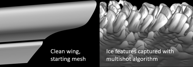
As ice accretes on aircraft surfaces, the geometry of the surfaces exposed to the incoming air and droplet flow changes, leading to changes of surface heat fluxes, collection efficiency, shear stresses, etc. In case of internal flows, ice can increase the blockage of passages between blades and other internal walls. To capture the effects of surface geometry change due to icing, the computational grid and the air and droplet solutions need to be updated frequently. The multishot icing approach splits the ice accretion duration into shorter sequential steady-state shots, modeling the unsteady ice accretion in a quasi-steady manner. The durations of the shots are user-defined. After each shot, the grid is updated either by morphing or by remeshing to conform to the new ice shape, also providing surface roughness information if the ICE3D beading model is enabled. The airflow solution is computed again using the previous shot’s solution as a restart. Similarly, the droplet and/or ice crystal solutions are updated and a new ICE3D solution follows. Multishot icing options are provided separately for FENSAP, Fluent, and CFX airflow solvers.
In a MULTI-FENSAP sequence, the computational grid is updated after the surface is displaced with ice at each shot. One of the mesh update methods available is to displace the node coordinates without changing the topology of the original grid. The other option is to remesh the surface and the volume to help maintain a proper surface grid resolution and quality and provide a better mesh for the next shot. In both cases, FENSAP, DROP3D, and ICE3D are executed in sequence followed by a grid displacement/remeshing step before moving onto the next shot. The following table lists the steps done at each shot.
Table 10.2: Solvers
| FENSAP | Will use the new displaced grid and its own air solution on the previous grid as a restart. |
| DROP3D | Will use the displaced grid, the new air solution from FENSAP and its own droplet solution on the previous grid as a restart. |
| ICE3D |
Will use the displaced grid, the new solutions from FENSAP and DROP3D. ICE3D itself will restart from the previous ice shape and surface icing solution automatically (film height, bead height, surface temperature, etc.), no manual setup option is necessary. |
| Grid Displacement |
The grid will be morphed or remeshed based on the type of grid displacement selected. Two options are available: for morphing the mesh with constant topology and to automatically remesh the entire grid using meshing journal files for Fluent. |
Tip: For guess-free, accurate computations of ice shapes, select the Beading model in the ICE3D config file (See Beading) to automatically transfer the spatially- and temporally-evolving roughness data to the airflow module at the end of each shot. The initial roughness height can be specified as a small constant value (k s≈0.5 mm), or from one of the various sand-grain roughness correlations provided by the FENSAP module. This initial value will be automatically overwritten after the end of the first shot.
The multishot procedure can also be started from a clean surface by specifying a sand-grain roughness height of zero, however a number of additional shots of short duration should be added to properly start the procedure.
The configuration of a multishot icing simulation uses FENSAP, DROP3D, and ICE3D configurations as building blocks, where each module is configured separately with the possibility of dragging and dropping the reference settings from one solver to the next. The shot duration is set in the main multishot configuration panel, but to facilitate the shot entries the total icing time in the ICE3D configuration can be set to the shot length intended. In this manner adding multishot iterations, or shots, will copy this time as the iteration (shot) length.
The mesh update options are found in the Out panel of the ICE3D configuration.
Using ALE Displacement to update the mesh by morphing significantly faster than remeshing since the topology and number of nodes remain constant and no solution interpolation between grids is necessary. However, not updating the grid topology has several limitations. Since the number of nodes remains constant, this method tends to coarsen the surface grid as ice accretes. Due to fixed mesh topology between shots, this method is not very effective in capturing complex glaze ice shapes. Due to these limitations, this approach often requires manual remeshing after a certain amount of automatic shots to maintain appropriate mesh and solution quality. However, this method is still able to capture rime ice shapes well since the ice shape usually conforms to the original shape of the aircraft surface.
The Remeshing – Fluent Meshing option is a sophisticated meshing method where wall boundary bridging, gap closing, and other geometry topology changes are supported. This option calls Fluent with a prescribed meshing journal file that is generic enough to deal with a wide range of mesh configurations. The remeshing step first executes a shell script that includes running Fluent and carrying out restart solution interpolations once the new grid is ready. To learn more about remeshing with Fluent Meshing, refer to Automatic Remeshing Using Fluent Meshing.
The MULTI-FLUENT sequence is defined around an initial Fluent case file (.cas(.h5)).
Double-click the input grid and select the initial Fluent .cas(.h5) file; the file should be in the same directory as the .dat(.h5) file with the initial solution.
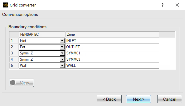
This operation will open the FLUENT-to-FENSAP Grid converter; this will convert the grid to the FENSAP format, for use with DROP3D and ICE3D.
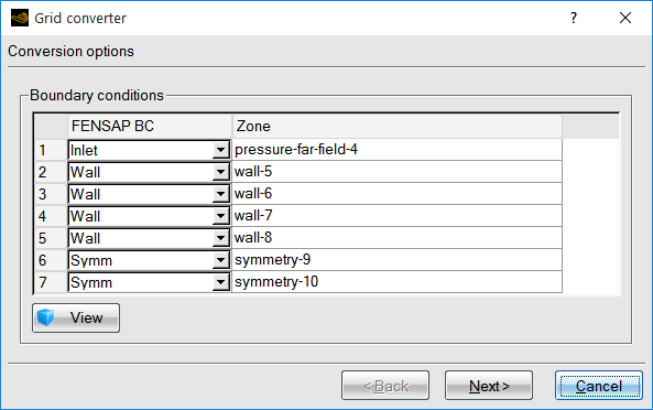
If the default choices for the boundary condition types are not suitable, select the correct FENSAP boundary condition type for each of the Fluent zones. In the next panel, the numerical parameters can be kept to their default values. When done, click Next.
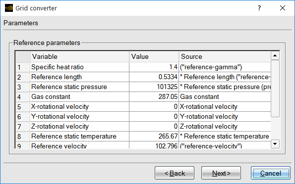
In the next panel, the Reference parameters can be kept to their default values, which are the Reference Conditions of Fluent, or modified. It is suggested to keep these default values if you followed the recommendations in Recommendations to Set up a Fluent Calculation regarding the setup of the Reference Conditions in Fluent.
The last panel will convert the grid to FENSAP format, the button helps to double-check the grid conversion and boundary condition types, using the internal 3D viewer.
All Fluent input parameters must be set up in the case (.cas(.h5)) file; FENSAP-ICE does not permit the modification of the Fluent input parameters.
The icon for the Fluent run will enable the selection of some Fluent-specific run parameters:
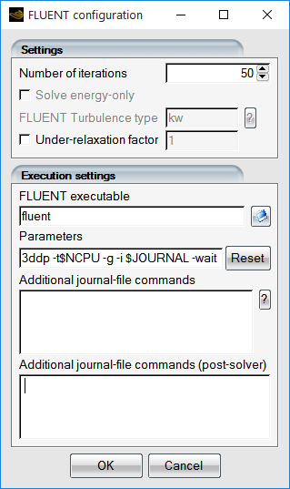
Table 10.3: Fluent Configuration Window
| Number of iterations | Fluent will execute for the specified number of iterations. |
| Solve energy-only | The journal file will contain a command to disable the flow and turbulence computation, however the FLUENT Turbulence type (if any) must be specified in the text box. |
| Under-relaxation factor | If specified, the Under-relaxation factor will be applied to the temperature computation. |
| FLUENT executable | Assuming that the default Fluent executable cannot be found in your $PATH environment variable, it allows the selection of the full path to the Fluent executable. |
| Parameters | The command line arguments used to launch Fluent. To use
the double-precision solver, use the 3ddp
flag instead of 3d flag. Do not remove the
–g –I $JOURNAL options.
In the Windows operating system, the
command line should also contain the
–wait flag. |
| Additional journal-file commands | For experienced Fluent users. Click the button for more information. |
This section provides recommendations for obtaining a steady-state airflow solution Fluent that is suitable for icing simulations with FENSAP-ICE. It outlines models, settings and inputs that will produce results as consistent as possible to those obtained with the FENSAP airflow solver that has been used in numerous validation cases for icing simulation predictions.
Inside your Fluent run:
Select General from the side menu and ensure the Solver is set to Type: Pressure-Based, Velocity-Formulation: Absolute and Time: Steady.
Select Models from the side menu.
Ensure that Energy is turned On.
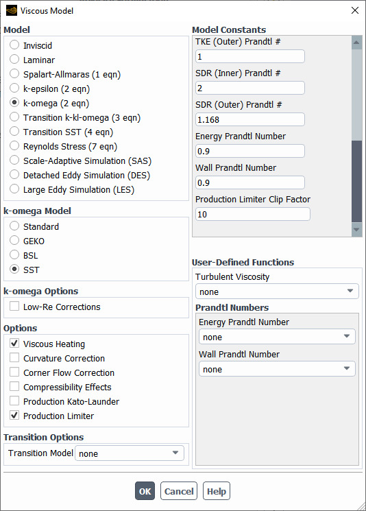
Under Viscous, change the Model to k-omega (2eqn) and then to SST under k-omega Model. To produce viscous effects as consistent as possible to those in the FENSAP airflow solver:
Enable Viscous-Heating and Production Limiter in the Options section.
Change the Energy Prandtl Number and Wall Prandtl Number to
0.9and the Production Limiter Clip Factor to10in the Model Constants section.
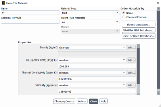
Select Materials from the side panel and, under Fluid, select air. By default, FENSAP models air as an ideal gas. Therefore,
Set the Density to ideal-gas.
Set the Cp (Specific Heat) (j/kg-k) to
1004.688J/kg/K. This value is equal to 7/2 R. In FENSAP, the gas constant R is 287.05376 J/kg/K.Set the Thermal Conductivity to constant. To compute its value, refer to The Energy Equation and replace T in the equation by the static ambient air temperature.
Set the Viscosity to constant. To compute its value, refer to The Continuity and Momentum Equations and replace T in the equation by the static ambient air temperature.
Note: If beading is disabled in ICE3D, the initial Fluent roughness settings will be preserved throughout the shots.
If the initial Fluent solution was computed using a serial or parallel solver execution, the same parallelization setting should be used in the subsequent multishot execution. Fluent might reorder the nodes of the grid, when switching between serial and parallel execution, making the reordered grid unsuitable for FENSAP-ICE restarts. You should always use the parallel version of Fluent, to avoid mismatches.
Under Boundary Conditions
On the inlets of the computational domain that represent ambient conditions:
Set the Turbulence Intensity to
0.08% (based on Effective Inflow Conditions for Turbulence Models in Aerodynamic Calculations paper by Philippe R. Spalart and Christopher L. Rumsey. "Effective Inflow Conditions for Turbulence Models in Aerodynamic Calculations", AIAA Journal, Vol. 45, No. 10 (2007), pp. 2544-2553.)Set the Turbulent Viscosity Ratio to
1e-05(consistent with FENSAP’s default Eddy/Laminar viscosity ratio).
On the walls that are prone to icing:
In the Momentum panel, set Shear Condition to No Slip and the Wall Roughness to High Roughness (Icing). Specify a Roughness Height equal to
0.0005mm in the Sand-Grain Roughness sub-panel to start your icing simulations. This height is automatically updated at every shot if beading is selected in ICE3D. For more information regarding the High Roughness (Icing) roughness model, consult Additional Roughness Models for Icing Simulations within the Fluent User's Guide.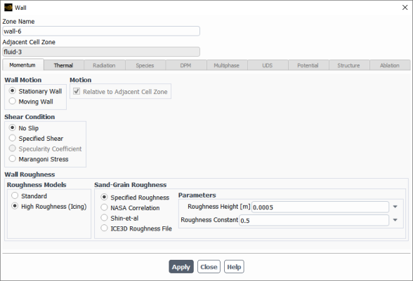
In the Thermal panel, set the Thermal Conditions to Temperature. Specify a Temperature equal to the Adiabatic stagnation temperature + 10 K. See Reference Conditions to compute this parameter.
Under Reference Conditions, use the ambient airflow properties to set the Reference Values. This provides consistency with the workflow of FENSAP-ICE and facilitates subsequent setup of DROP3D, ICE3D and CHT3D calculations since these Reference Values must be used as Reference parameters during the Fluent to FENSAP format conversion (See Fluent Configuration) and as Reference Conditions in the Conditions panel of DROP3D or an ICE3D simulations.
Under Solution Methods, you should set the Pressure-Velocity Coupling scheme to Coupled and to select at least a Second Order or Second Order Upwind scheme for the Spatial Discretization of the governing equations.
Monitor your solutions, especially surface static pressures, shear stresses and convective heat fluxes. It is important to obtain smooth continuous solutions of these fields as they play a major role during ice accretion.
DROP3D can accept the converted Fluent airflow solution as input; however the correct reference conditions and other physical quantities must be provided to DROP3D and ICE3D, and must be identical to those specified for the Fluent solution. FENSAP-ICE does not automate this process; these values must be defined manually and you must ensure their correctness.
If you followed the recommendations in Recommendations to Set up a Fluent Calculation, the correct reference air conditions in DROP3D and ICE3D should have been automatically populated in these simulations.
The multishot configuration is similar to that for FENSAP-DROP3D-ICE3D. However, the Fluent run can be set up for a different number of iterations for each step:
Use and select the FLUENT - FLUENT-iterations variable.
When Fluent is executed, the log will be available in the run panel of FENSAP-ICE:
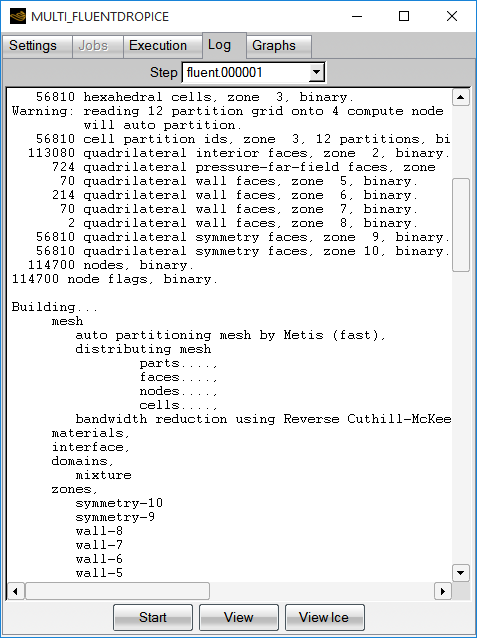
The Fluent output file will be named OUT.dat, and then the file will be renamed to an iteration-specific file name and converted to FENSAP format.
The following files will be created at each multishot iteration:
soln.fluent.00000X.cas
soln.fluent.00000X.dat
soln.fluent.00000X
The MULTI-CFX sequence is defined around an initial CFX .res file.
Double-click the input grid and select the initial CFX .res file.
This operation will open the CFX-to-FENSAP Grid converter, which will convert the grid to FENSAP format for use with DROP3D and ICE3D.
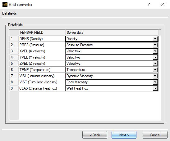
If the default choices for the boundary condition types are not suitable, select the correct FENSAP boundary condition type for each of the CFX zones. In the next panel, the Datafields parameters can be kept to their default values. Click .
Note: If you are performing a MULTI-CFX simulation using automatic remeshing with Fluent Meshing, there are additional requirements for the boundary and domain names that should be used in the CFX setup. Refer to the note related to CFX in Automatic Remeshing Using Fluent Meshing.
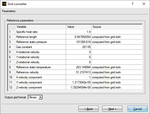
In the next panel, the Reference parameters can be kept to their default values or modified. It is suggested to keep these default values if you followed the Recommendations to Set up a CFX Calculation.
The last panel will convert the grid to FENSAP format, the button allows you to double-check the grid conversion and boundary condition types, using the internal 3D viewer.
All CFX input parameters should have already been set up in the .res file; FENSAP-ICE does not permit the modification of the CFX input parameters.
Note: Only execution parameters can be modified.
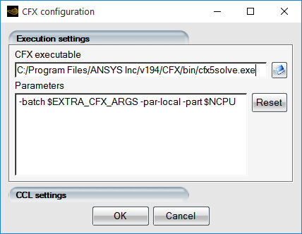
| CFX Executable | This allows the selection of the full path to the CFX executable, when the default CFX executable cannot be found in your $PATH environment variable. |
| Parameters |
This section describes the command line arguments used to launch CFX in batch mode, -batch flag. The flag -par-local indicates that the CFX simulation will use the local host parallel CPUs or processors. The $NCPU indicates the number of processors employed. The value of NCPU is taken from the number of CPUs specified in Execution Settings of your multishot configuration. EXTRA_CFX_ARGS (Optional): If an environment variable has been defined, the $EXTRA_CFX_ARGS will be replaced by its value. For more details on the CFX command line, refer to Command-Line Options and Keywords for cfx5solve in the CFX-Solver Manager User's Guide. |
| CCL Settings |
For experienced CFX users. |
This section provides recommendations for obtaining a steady-state CFX airflow solution that is suitable for icing simulations with FENSAP-ICE. It outlines models, settings and inputs that will produce results as consistent as possible to those obtained with FENSAP, the airflow solver of FENSAP-ICE that has been widely used in numerous icing validation cases.
Inside your CFX run:
In the top menu bar, go to and select . In → → → , check mark .
For every CFD Domain located on the side menu bar under Simulation → Flow Analysis, right-click the domain name and select to modify the following sub-menus:
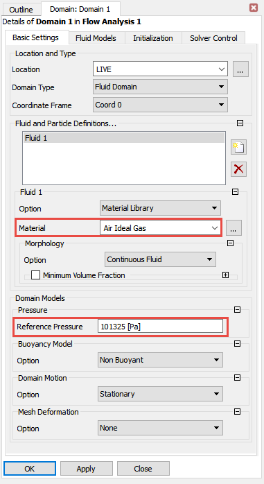
Inside Basic Settings:
Select as the Material of your Fluid Domain. By default, FENSAP models air as an ideal gas.
Use the ambient static pressure of your simulation as Reference Pressure.
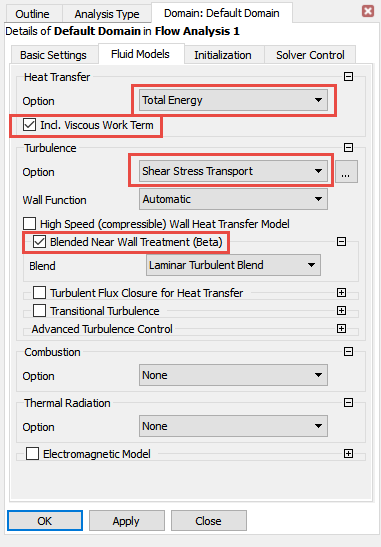
Inside Fluid Models:
Select and activate under Heat Transfer.
Select and checkmark under Turbulence.
If the bounding region of your CFD Domain is an Inlet that represents ambient conditions:
In the Boundary Details panel, set Turbulence → Option to .
Set Fractional Intensity to
0.0008(based on Effective Inflow Conditions for Turbulence Models in Aerodynamic Calculations paper by Philippe R. Spalart and Christopher L. Rumsey. "Effective Inflow Conditions for Turbulence Models in Aerodynamic Calculations", AIAA Journal, Vol. 45, No. 10 (2007), pp. 2544-2553.).Set the Eddy Viscosity Ratio to
1e-05(consistent with FENSAP’s default Eddy/Laminar viscosity ratio).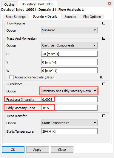
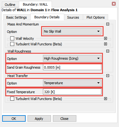
If the bounding region of your CFD Domain is a Wall that is prone to icing:
In the Boundary Details panel, set the Mass And Momentum to No Slip Wall.
Set the Wall Roughness to High Roughness (Icing) and specify a Sand Grain Roughness height equal to
0.5mm to start your icing simulation. This height is automatically updated at every shot if beading is selected in ICE3D. Otherwise, it is preserved. For more information regarding the High Roughness (Icing) roughness model, consult Wall Roughness.Set the Heat Transfer to and specify a Fixed Temperature equal to the Adiabatic stagnation temperature + 10 K. See Reference Conditions to compute this parameter.
On the side menu bar panel, you should use the following solver settings located in Simulation → Flow Analysis → Solver → and double-clicking Solver Control.
Inside Basic Settings:
Set the Advection Scheme and Turbulence Numerics to .
Keep the default settings of the Fluid Timescale Control. The default settings should be for the Timescale Control, for the Length Scale Option and a Timescale Factor of
1.0.Under Convergence Criteria, set its Residual Type to and its Residual Target to
1e-20to promote convergence.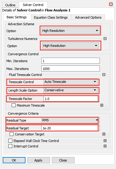
Inside Equations Class Settings:
If oscillations of shear stress and heat flux are observed on the Walls of the Domain and if the cause of these oscillations is not linked to the geometry or the mesh refinement of the CFD simulation, you should change the of the turbulence and energy equations to Local Timescale Factor and to use a factor of
1or a factor below5.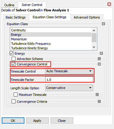
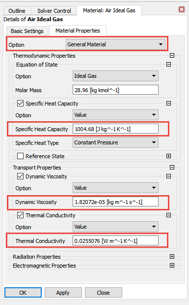
On the side menu bar panel, double-click the default Air Ideal Gas properties located under Simulation → Materials.
Inside Basic Settings:
Set air as a with Material Group equal to .
Inside Material Properties:
Select under Option.
Specify the following Thermodynamic Properties:
In the sub-menu, specify the Specific Heat Capacity to
1004.688J/kg/K and the Specific Heat Type to . The value of the specific heat capacity at constant pressure is equal to 7/2 R. In FENSAP, the gas constant R is 287.05376 J/kg/K.In the Transport Properties sub-menu, use The Continuity and Momentum Equations to compute the Dynamic Viscosity and The Energy Equation to compute the Thermal Conductivity. In both equations, replace T by the static ambient air temperature.
On the top menu bar, select Execution Control, and select in the Run Definition panel.
CFX does not have a menu to define reference airflow conditions. Therefore, during the CFX to FENSAP format conversion, inlet airflow boundary conditions and/or solution are automatically selected by the graphical user interface of FENSAP-ICE as reference conditions. However, to set the reference pressure condition, specify its value inside the Reference Pressure field located in the Domain panel of CFX. In general, the airflow reference conditions should correspond to the ambient airflow properties of the CFD simulation. If this is not the case, new reference conditions can be defined during the CFX to FENSAP file conversion. See Input Grid Configuration.
Monitor your solutions, especially surface static pressures, shear stresses and convective heat fluxes. It is important to obtain smooth, continuous solutions of these fields as they play a major role during ice accretion. See the Solver Control recommendations located at Recommendations to Set up a CFX Calculation.
Note: If you are performing a MULTI-CFX simulation using automatic remeshing with Fluent Meshing, there are additional requirements for the boundary and domain names that should be used in the CFX setup. Refer to the note related to CFX in Automatic Remeshing Using Fluent Meshing.
DROP3D can accept the converted CFX airflow solution as input; however, correct reference conditions and other physical quantities of air must be provided to DROP3D and ICE3D. The default airflow parameters suggested by DROP3D and ICE3D are not the most appropriate for your icing simulation. If you followed the recommendations in Recommendations to Set up a CFX Calculation, the correct reference air conditions in DROP3D and ICE3D should have been automatically populated otherwise, you should use the ambient airflow conditions to manually define the reference conditions and other physical quantities of air inside DROP3D and ICE3D.
The multishot configuration is similar to that for FENSAP-DROP3D-ICE3D, however, the CFX settings cannot be modified at each shot through this configuration panel. Therefore, the original CFX settings are preserved during the entire multishot calculation.
When CFX is executed, the log will be available in the run panel of FENSAP-ICE:
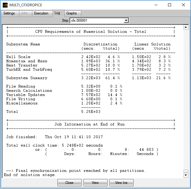
CFX output files will be named using an iteration-specific suffix that considers the shot number. These files will then be converted to FENSAP format.
The following files will be created at each shot:
soln.cfx.00000X.res is the CFX airflow solution file in CFX format.
soln.cfx.00000X.disp.res is the CFX displaced mesh solution file in CFX format.
soln.cfx.00000X is the CFX airflow solution file in FENSAP format.
grid.ice.00000X is the CFX displaced mesh solution file in FENSAP format.
All .res files in the graphical user interface of FENSAP-ICE can be post-processed using CFD-Post by right-clicking the CFX solution and by selecting and then . The airflow solution, converted to FENSAP format, as well as the other DROP3D and ICE3D output files can be visualized using Viewmerical.
For multishot cases, where the ice shape growth is significantly large such that the original mesh and surface topology can no longer be deformed or maintained, the iced surface should be remeshed. By default, remeshing is done using Fluent Meshing. In this case, a journal file that combines the ice STL file created by ICE3D and the original grid file for the case is employed. Alternatively, one can write a custom remeshing script to be used with a third-party mesher. The first section below describes this remeshing process with Fluent Meshing.
Fluent Meshing is a powerful meshing tool with the possibility of automation and scripting of complex meshing operations. It can mesh ice surfaces with challenging topologies.
Example Fluent remeshing scripts to replace the grid displacement steps of MULTI-FENSAP and MULTI-FLUENT and MULTI-CFX simulations are provided in the data/templates/remeshing directory of the FENSAP-ICE installation folder. Depending on the simulation type and operating system, the appropriate files are automatically copied to the run directory. These script files are named custom_remeshing.sh, and are tagged for use with FENSAP, Fluent and CFX airflow solvers as well as with Windows and Linux operating systems. In these example scripts, Fluent Meshing is called with a journal file to perform the remeshing procedure. The journal file, named remeshing.jou, controls the remeshing steps using a very generalized and automated meshing technique. Additionally, the journal file calls a meshingSizes.scm file, which contains required case specific meshing parameters, such as minimum and maximum element sizes. Finally, a remeshing.wft file is included to support future developments related to Fluent remeshing workflows. These example journal and sizing files are also located in the data/templates/remeshing directory.
To use this remeshing procedure with Fluent Meshing, choose in the grid displacement menu and switch the Template to .
Based on your needs and experience with Fluent Meshing, the journal file can be enhanced and customized to include more specialized sizing functions, refinement zones bodies of influence, hard-set mesh sizing for certain boundaries, etc. In its most basic form, the provided journal file should be able to handle long duration glaze icing cases for external icing simulations on wings, nacelles, multi-element airfoils, complete aircraft configurations, etc., provided that you properly determine the meshing sizes that will prevent the collapse of sharp features like trailing edges.
Note:
The mesh size will increase from shot to shot due to the growth of the iced layer and the smallest size function that is being used in these areas. This should be considered before launching a multishot calculation and computational resources in terms of CPUs, memory, and disk space should be adjusted.
Walls should be separated into different zones at corners or joints. Doing so will ensure, sharp edges of the geometrical model will be preserved after wrapping. For example, if the tip cap of a wing is placed in the same boundary family as the rest of the wing, the corners will be smoothed during the wrapping operation, which should be avoided.
Grid file format conversions are carried out using
fluent2fensapandfensap2fluentcommand line tools. The-zonebcoption should be used during conversions to maintain FENSAP boundary condition family IDs by converting them to zone#### format in the *.cas(.h5) file and back to 4 digit #### format in the FENSAP grid file. Otherwise, the FENSAP boundary IDs may get reshuffled, resulting in incorrect settings for the next shot.When using Fluent as the airflow solver with this custom remeshing script, in your initial .cas(.h5) file, you must first edit your boundary names to the zone#### format. Make sure to use FENSAP boundary conditions numbering format inside the Fluent case file (for example, zone1000 for inlets, zone2000 for walls, zone3000 for exits, zone4000 for symmetry and zone5000 for periodic boundaries). Without these names, the remeshing journal file will not generate a 3D mesh.
During a multishot simulation the custom_remeshing.sh script will perform the following operations:
Convert the script inputs ($grid_input, $grid_next…) to simple variables to be used throughout the script.
Extract the previous and next shot numbers (ex: 000002, 000003) from these variables.
Clean up and remove any files that exist from previous simulations.
Create a shell.cas file containing all boundaries from the initial mesh that will be used during the remeshing operation.
Copy the most recent iced geometry STL file to a general ice.stl name for use during the remeshing operation.
Call Fluent Meshing with the remeshing.jou journal file to perform the remeshing operation, creating a new mesh (newmesh.cas).
Convert the newmesh.cas file to FENSAP format, using the -zonebc option to preserve FENSAP boundary family IDs.
[Optional]: Interpolate the FENSAP and DROP3D results of previous shot to the new mesh to be used as restarts. This is skipped if multishot Iteration restart is set to mode
Interpolate roughness and screen wire diameter profiles onto the new mesh.
Ice Smoothing During Multishot With Remeshing
For some cases, nonuniformities in the ice shape growth at wall intersections can lead to failures in the wrapping process of Fluent Meshing. These issues are mostly observed in internal icing cases, such as engine inlet guide vanes where the ice that grows on the blade, can eventually fold towards the hub and shroud surfaces and lead to a variety of meshing problems. The ice smoothing option provided in the Icing model panel can be used to help with this situation. The following example shows a 10-shot icing simulation with remeshing on an IGV which fails without the ice smoothing option. The solution using 3 ice smoothing iterations still maintains the glaze ice horns, while having less surface oscillations.
Requirements for MULTI-CFX Runs
When using CFX as the airflow solver with this custom remeshing script, you must modify your initial .res file in CFX-Pre.
Make sure that only one 3D region/domain exists in your .res file. The current MULTI-CFX supports only one domain for external icing simulations.
Note: If you would like to use the geometry from a multi-domain mesh, it is recommended to go back to the tool used to generate the mesh and create a new mesh with a single domain represented by a continuous fluid domain.
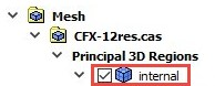
Change the Principal 3D Regions names to .
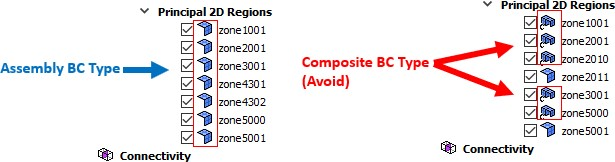
Make sure that all BCs under Principle 2D Regions are Assembly BC type; the Composite BC type of CFX is not supported. In case there are Composite BC types in your .res file, you may need to re-define their BC type in your meshing process or
Import the CFX mesh within Fluent, → →
Save the file as .cas, →
Note: You may need to execute the cmd in Fluent's TUI to be able to write the .cas file format: /file/cff-files
Reload the file within CFX-Pre, → →
to change the BC type from composite to assembly.
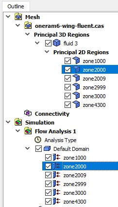
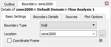
Set the Principle 2D Regions names and Boundary names to the zone#### format. Make sure to use FENSAP’s boundary conditions numbering format (for example, zone1000s for inlets, zone2000s for walls, zone3000s for exits, zone4000s for symmetry). Each Boundary name must be linked only to its corresponding Principle 2D Regions with the same name. For example, if you have a wall boundary with Boundary name zone2000, in its Basic Settings → Location, the Principle 2D Region, also called , must be selected.
MULTI-CFX supports only one pair of periodic BCs in a 3D external region/domain. Periodic BCs must be named as zone5000 and zone5001. When your .res file has Interfaces with periodic BCs, you must change your periodic interface’s name to , and re-name the two corresponding BCs as
zone5000andzone5001under Principle 2D Region. Then, make sure that the two Periodic Sides of Interfaces Periodic are referring them, respectively.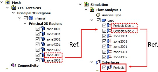
The custom remeshing scripts are set to use the AWP_ROOT221 environment variable to launch Ansys tools. This variable is automatically set by the Ansys installer as the default Ansys directory. However, if this is incorrect, you may correct this variable in your environment before launching FENSAP-ICE, or in your custom_remeshing.sh script (for example:
export
                            AWP_ROOT221=/path/to/ansys_inc/v221/
).
Using Custom Fluent Meshing Journal Files
Based on user needs and their experience with Fluent Meshing, the journal file can be enhanced and customized to include more specialized sizing functions, refinement zones bodies of influence, hard-set mesh sizing for certain boundaries, etc. There are currently two recommended ways to manage adding these enhancements to the remeshing journal files.
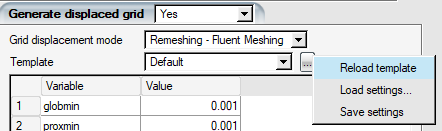
The first option it select the Template -> Default option, which will copy the default remeshing.jou files to the current run directory. Next, a user can open the remeshing.jou file and add any modifications required to the Fluent remeshing script. This option may be preferred if the user would like to make quick adjustments to the default template for use in the run of interest. However, in this case the UI Template option will still be listed as Default, so care should be taken when setting up new runs in the same project to ensure the proper file is used in each run. For example, if a user drag and drop’s the configuration from a run containing a modified default remeshing.jou template, the modified remeshing.jou file will be copied to the new run’s directory. To reload the default template, select () → to the right of the Template option box.
A second option is to setup a custom remeshing script and load it into the run. First, create a remeshing_templates folder inside the simulation project directory. Next, place the following files into your remeshing_templates folder:
customname.wft: this file is required so that the template can be automatically recognized by the UI. For now, it can simply be an empty text file. (In the future, this file will allow for further Fluent meshing workflow developments).
customname.jou: this file should contain the complete Fluent Meshing journal commands to perform the remeshing operation within Fluent Meshing.
customname-meshingSizes.scm: this file should contain the mesh size information requested by the user. It will be loaded into the table accessible inside the UI, and accessed by the journal file above during the remeshing process.
Note: The customname portion of the filenames above can be whatever the user desires, it is simply a requirement that the same string is used.
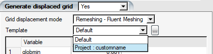
Once the files above are placed in the remeshing_templates folder, they will then be accessible inside the Template selection box. Choosing the custom template will copy the files into the current run. If the custom template is at first not available, close and then re-open the ice config to have the user interface auto-check for new remeshing templates.
Multishot with remeshing requires you to configure numerous model and meshing parameters, each of which can significantly impact the outcome depending on the icing conditions and the geometry being iced. The following guidelines were developed through the AIAA Ice Prediction Workshop efforts and various complex icing scenarios, including full-scale aircraft with multiple components.
Initial Mesh
The remeshing journal used with Fluent Meshing is configured to compute a surface sizing function based on curvature and proximity. The curvature sizing by default uses a 5 degree facet-to-facet criterion to constrain the edge size during the shrink-wrap process. The initial grids should also respect this criterion especially on boundaries where icing is enabled. If the initial grid has a coarser surface curvature, for example, 10 degree separation between facets, excessive refinement on such zones may occur along the initial grid lines. This will manifest as oscillations in collection efficiency and heat fluxes, which is likely to imprint on the ice shape.
Before version 2025 R2, wall boundaries had to be split along sharp features that needed to be preserved. These can be trailing edges, sharp or blunt, wing/body joints, etc. This is no longer a requirement, the latest version of the remeshing journal can detect these features and use them for wrapping imprint, even if the boundaries are merged. Keeping major components in separate boundary families is still a recommended practice as it would make post processing and data reporting simpler. Wings, fuselages, tails, nacelles, pylons, etc. can be stored in individual boundary families.
The icing model uses wall-resolved boundary layers to extract heat transfer coefficients. The boundary layers are also important in correctly capturing droplet impingement limits in the Eulerian approach. Keeping y+ ~ 1 is recommended, with an initial cell height in the order of 1e-6 to 1e-5 meters. Small geometries like air data probes, antennas, and turbomachinery components can be meshed with an initial cell height of 1e-6 m. Large aircraft components could use higher initial cell sizes, not exceeding 1e-5 meters. You should do a boundary layer refinement study and check the rough (0.5mm to 1.0mm sand grain roughness) heat flux convergence with initial cell size, focusing on areas where icing is expected. Heat transfer coefficient (HTC), along with collection efficiency, is the main driver of the icing process which will determine the type of ice, as in rime, glaze, or mixed.
Meshing Sizes
Meshing sizes should be set considering the overall size of the geometry, curvature and proximity of the geometry, and the mesh size that can be afforded with the available computational resources. If the minimum sizes in the remeshing setup are kept too low, the mesh size can grow very rapidly to impractical levels. Global minimum and proximity minimum should be set low enough to capture the spacing between surfaces that meet at a blunt trailing edge. Wing trailing edges, aircraft fuselage tailcone closing surfaces, etc. are the usual places to examine when evaluting proximity minimum size. Sharp trailing edges are not affected by this, as the edge that makes the sharp edge will be imprinted as expected even if the mesh size is large.
Minimum curvature sizing can be set in a range of 1mm to 5mm for external icing applications on main aircraft components like the wings, nacelles, tails, etc. The results shown by Ansys in the 2nd Ice Prediction Workshop (IPW2) on the CRM65 wing sections were computed using 2mm edges. If running a full scale aircraft simulation (for example, wing semi-span ~ 30m), 3mm curvature minimum size would be the corresponding scale to what was used for CRM65 simulations with 2mm edges in the IPW2. You should be aware that with this setting of 3mm, a 30m semi-span wing will end up with 100-150 million mesh nodes, or over 400 million cells. Using a coarser setting like 5mm can save a lot of mesh points, while reducing the ice shape fidelity, but still maintaining most of the 3D features.
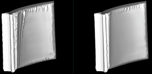
The following image compares the the 10-shot ice shape computed on the CRM-HL wing around the mid-span region, using 3mm (top) and 5mm (bottom) minimum mesh sizes:
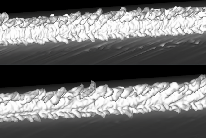
Here, the case with a 3 mm edge size reached 350 million cells by shot 10, while the case with a 5 mm edge size reached 200 million cells. The figure below compares ice traces from the two runs:
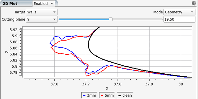
With scalloped ice shapes like this, it will not be possible to match the traces exactly between two runs with different sizing settings. The ice shapes from these cuts are very similar despite the 3D effects and the mesh resolution.
For smaller components like air data probes and turbomachinery blades, minimum sizes can be in the order of 0.1mm. Fan and compressor blades are usually less than a millimeter thick at the blade tips. You will lose blade definition of the minimum sizes are larger than the blade thicknesses.
When simulating cases with wind tunnel walls, these walls will also use the proximity and curvature sizing limits. Maximum edge size on tunnel walls will be limited to curvmax. You may want to keep this high and equal to globmax, not to over-refine the tunnel walls away from the test article.
Number of Shots
Number of shots dividing the whole icing duration has a strong effect on the ice shape outcome. The detailed 3D ice shapes require 10-15 shots. Rime ice shapes which are less detailed could be done with less shots. If ice shapes are not required in high fidelity, glaze ice cases can be done with 3-5 shots just to get the overall shape without details of scallops. The number of shots to use in an analysis is ultimately a factor of application and the end goal of the analysis. If scallop details are required in a swept wing icing study, then this can be obtained with 10 shots. If overall ice mass and a low-fidelity (smooth) ice shape is enough, then 3-5 shots can be used.
Currently there is no formalized way of determining number of shots or shot lengths, but the following could be considered as a guide. Usually ice shapes are reported in minutes, and not with fractions of seconds. For practical reasons, dividing the icing time to equal lengths in minutes and staying in the range of 10-15 shots for high fidelity, and less or equal to 5 for low fidelity is reasonable. If starting with a clean surface (sand grain roughness = 0), the first shot can be split into two parts with the first part being a short duration to build some roughness with the beading model. For example, for a 45 minute ice accretion simulation on a wing, you could do 9 shots of 5 minutes each, starting with some nominal roughness like 0.5mm, or 10 shots with the first two being 1 and 4 minutes, and the remaining 8 shots 5 minutes each, if doing the first shot with zero roughness. The figure below shows the results of 20 shots (left) and 3 shots (center) for Case 362 of IPW1:
The 20-shot ice shape is very detailed compared to the 3-shot ice shape, but the ice trace comparison on the right shows that the two shapes are similar in terms of size and coverage.
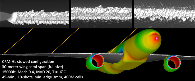
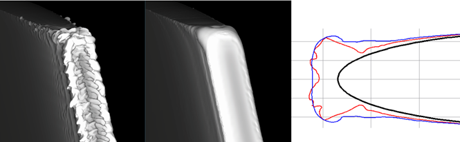
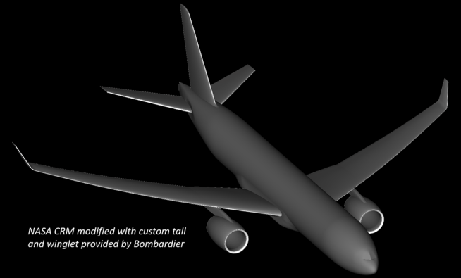
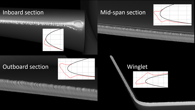
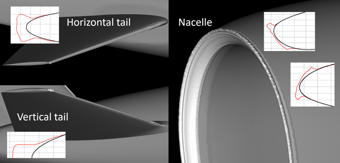
The next sequence of figures show a 5-shot low-fidelity icing case on a modified CRM geometry with winglets added. The shots are organized as 5min + 4x10min, with the first shot using zero roughness in airflow and building roughness with the beading model. Ice smoothing was also enabled to defeature the ice shapes, to keep the mesh count relatively low. Icing conditions are 45-minutes in App-C at 15000ft, with MVD 20 microns at T = -6°C. The shot 1 and shot 5 grid sizes are 125 million and 200 million cells, respectively. The ice trace graphs attached with each figure shows the classic dual horn ice shapes except at the inboard section where collection is low. This case is an example to using FENSAP-ICE in a computationally efficient way, not ending up with highly detailed ice shapes on every surface when simulating full scale airplanes with multiple components. If this case was calculated with 10 shots and no ice smoothing, the mesh count would have reached close to a billion cells which may be unnecessary for the end application.
Special Options for Very Large Grids
FENSAP-ICE performs some tasks like solution read/write, solution interpolation from previous shot’s grid to the next, on the head node of a job running on a computing cluster. As the mesh size increases, these operations become more taxing on the available memory of the head node. The interpolation step carried out by the soln2soln executable will fail if there is not enough memory. FENSAP modules may also fail when reading in a very large soln file. There are two options that can be used to delay the onset of these memory related issues.
The first one is the Write all variables option in FENSAP's Out panel. This can be disabled to reduce the output soln file size by removing some of the non-essential field variables like u+ and y+, Gresho heat flux, and turbulence variables. Turbulent viscosity and conductivity are always written since they are needed for particle thermal energy and vapor transport systems in DROP3D.
The second option is which is one of the choices under in the main multishot configuration window. When set, solution interpolations from the previous grid to the next will be skipped, avoiding the soln2soln execution.
Fluent Meshing can also run into problems when there is insufficient memory, either at the tetra meshing step or the mesh output step. This is best avoided by distributing the parallel fluent memory across the compute nodes of the job. This can be done by passing the machine file to Fluent Meshing in the remeshing script, by including it in the FLUENT_PARAMS environment variable in the job submission script. Starting with version 2025 R2, this is automatically done when the scheduler is set to SLURM, with the following lines being included in the submit script:
srun hostname -s | sort -u > slurm.hosts
export FLUENT_AFFINITY=0
export SLURM_ENABLED=1
export SCHEDULER_TIGHT_COUPLING=1
export FLUENT_PARAMS="-cnf=slurm.hosts"
FLUENT_PARAMS is used in the custom_remeshing.sh script as an argument to the Fluent batch execution command. For other schedulers like PBS, you would have to do something similar based on your system configuration, and add similar lines in the scheduler configuration panel of FENSAP-ICE run window.
It is possible to provide a custom prepared remeshing script for all the above described multishot icing simulations if desired. With a custom remeshing script, a user can sequence a grid generation procedure to be executed in batch with their preferred meshing tool, using the ice surface STL grid files as CAD inputs over the original surfaces.
The Custom_remeshing.sh script for remeshing with Fluent can be used as is for the most part to take care of file input, output, and solution interpolation steps. One can replace the grid conversion and Fluent execution lines and make sure that the new grid is properly converted to FENSAP format, keeping the same boundary condition names.
Such a script should be designed to perform the following steps:
Copy the last STL file (for example, ice.ice.000005.stl) generated by ICE3D to a common temporary name (for example, ice.stl).
Execute a meshing software that loads the base grid, the ice.stl file, and replaces the walls with those from the STL file, and fully or partially remeshes the grid.
Convert the grid to FENSAP format.
Interpolate air and droplet solutions from the previous grid to the new grid to serve as restart solutions.
Interpolate the surface roughness file from the previous grid to the new grid.
Perform cleanup and error checking operations along the way to stop the execution if an error occurs.
The option can be activated in the Out panel of the ICE3D configuration of a multishot simulation. When mode is used, the grid displacement step of the multishot simulation will be replaced with the line provided in the Remesh command, as shown in the figure below.
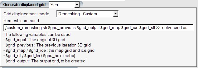
The first item in the Remesh command above specifies the bash script file used to control the custom remeshing procedure. This must be provided by the user and placed inside the run directory. Following this, there are a number of shell variables that will be used inside the script. These shell variables are available in the mode to allow the user to access the grid files necessary to perform the remeshing procedure. These variables will automatically contain the correct shot number associated with the previous or next shot of the multishot simulation. Inside the user’s custom remeshing script, the shot number can also be extracted from these names using standard bash script commands. The following variables are available to the user:
$grid_input: contains the name of the initial grid used in the multishot ice accretion simulation (for example, airfoilgrid.grd)
$grid_previous: contains the file name of the grid used in the previous shot of icing (for example, grid.ice.000002)
$grid_output: contains the file name of the grid that will be used in the next shot of icing (for example, grid.ice.000003)
$grid_map / $grid_ice: contains the file names of the map and ice grids used by ICE3D in the previous shot of ice accretion (for example, map.grid.ice.000002, ice.grid.ice.000002)
$grid_stl / $grid_tin: contains the file names of the stl and ICEM format CAD files produced by the previous shot of ice accretion (for example, ice.ice.000002.stl, ice.ice.000002.tin)
$grid_bc: contains the file names of the boundary condition files used in the previous shot of ice accretion (for example, timebc.dat.ice.00002)