


(Part A) Set up and process a simulation that makes use of Custom Fibers, defined by a .csv file. Use a Particle Custom Inlet together with Custom Fibers and Frozen Segments, to set the grass Fiber positions.
(Part B) Use Particle Mass to view how a Fiber breaks, calculate the Mower Blades’ Power and Torque and identify which regions of the blades are most susceptible to wear.
The main purpose of this tutorial is to learn to set up and process a simulation that makes use of Custom Fibers defined with Frozen Segments.
The scenario considered in this tutorial is a Lawn Mower cutting grass, where the individual grass plants are represented by Custom Fibers with Frozen Segments where the fibers attach to the ground.
You will learn how to:
Define a Custom Fiber particle shape using a .csv file
Export a particle shape to an .stl file
Use a Particle Custom Inlet, together with Custom Fibers and Frozen Segments, to set the grass Fiber positions
Attach the grass Fibers to a Motion Frame
And you will use these features:
Particle Custom Inlet
Custom Fiber Particle Shape
Multi-Element (Flexible) Particles
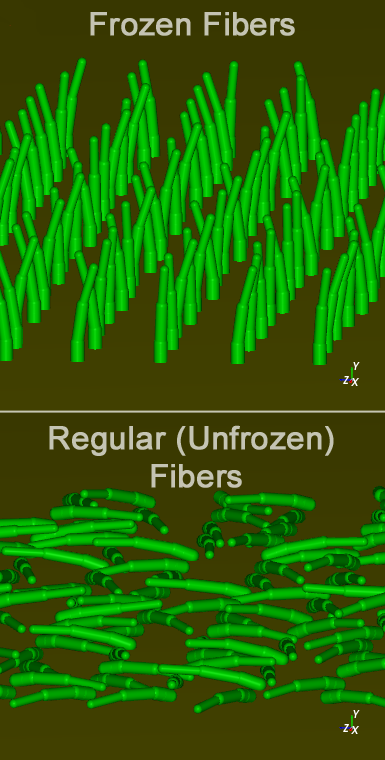
Frozen Fibers
Joint Breakage
Particle Shape Export
Important: This ADVANCED tutorial contains fewer details, screenshots, and procedures than other Rocky tutorials.
An ADVANCED tutorial is designed for users who are more familiar with the Rocky user interface (UI), and already have a good understanding of the common setup and post-processing tasks.
If you do not already have this level of familiarity, it is recommended that you complete at least Tutorials 01 - 05 before beginning this one.
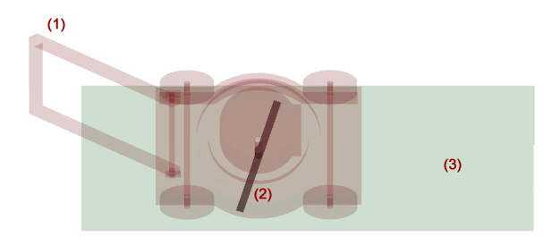
The geometries in this tutorial are composed of:
(1) Mower
(2) Blades
(3) Ground
These 3 items will be imported as .stl files, which can be found in the tutorial directory.
To get started with this tutorial, do the following:
Download the
dem_tut22_files.zipfile here .Unzip
dem_tut22_files.zipto your working directory.Open Rocky 2025 R2.
Create a new project.
Save the empty project to a location of your choosing.
Use the information in the tables that follow to start setting up your Rocky project.
Tip: If you run into settings or procedures in these tables that you are not yet familiar with, please refer to the Rocky User Manual and/or other Tutorials (via the Introductory Tutorials and Advanced Tutorials) to find the detailed instructions you need.
Step Data Entity Editors Location Parameter or Action Settings A Study Study Study Name Lawn Mower B Physics Physics | Momentum Numerical Softening Factor 0.1 [ - ] C Modules Modules Boundary Collision Statistics (Enabled) D Modules ﹂Boundary Collision Statistics
Boundary Collision Statistics Intensities (Enabled) E Geometries Import Wall blades.stl, ground.stl and mower.stl with "mm" for Import Unit F Geometries ﹂blades
Wall | Transform Translation 0, 0.005, 0 [m] Triangle Size 0.01 [m] G Motion Frames Create Motion Frame H Motion Frames ﹂Frame <01>
Frame Name Translation Add motion Velocity -0.17, 0, 0 [m/s] I Geometries ﹂ground
Wall Motion Frame Translation ⯆ J Motion Frames Create Motion Frame K Motion Frames ﹂Frame <01>
Frame Name Rotation Relative Position 0.185, 0, 0 [m] Add motion Type Rotation ⯆ Initial Angular Velocity 0, -30, 0 [rad/s] L Geometries Wall Motion Frame Rotation ⯆ M Materials ﹂Default Particles
Material Bulk Density 439 [kg/m3] Young's Modulus 1e+07 [N/m2]
For the Particles step, we will create a Custom Fiber, which is defined in a .txt or .csv file and then imported into Rocky.
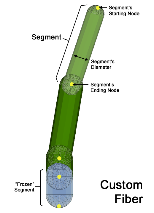
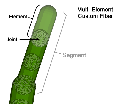
Custom Fiber shapes are made up of separate but connected Segments, which the positions are defined by the coordinates of each starting and ending Nodes.
Other properties can be defined per Segment, including its Diameter and whether or not the Segment will be considered Frozen.
In this tutorial, we will create a Custom Fiber with four segments of different diameters, which the bottom segment is Frozen (as shown).
The structure of the .csv file we will use to define this shape is shown below:
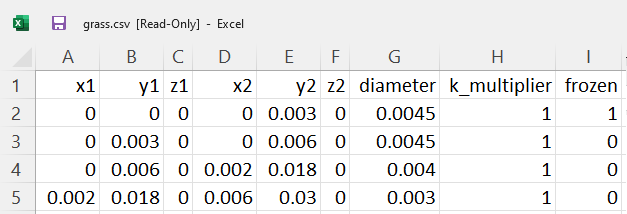
Each row beneath the header defines a separate segment where:
x1, y1 and z1 are the coordinates of the node that starts the segment.
x2, y2 and z2 are the coordinates of the node that ends the segment.
diameter is the segment's diameter.
k_multiplier (optional) is the Young's modulus multiplier for the segment.
frozen (optional) indicates whether the segment will be treated as frozen (1) or unfrozen (0).
Note: Segments of a multi-element Fiber defined as frozen will "stick" to a certain location and have only the unfrozen segments of the Fiber respond to interactions from other objects in the simulation.
Let's now create a Custom Fiber and import the .csv file that defines it.
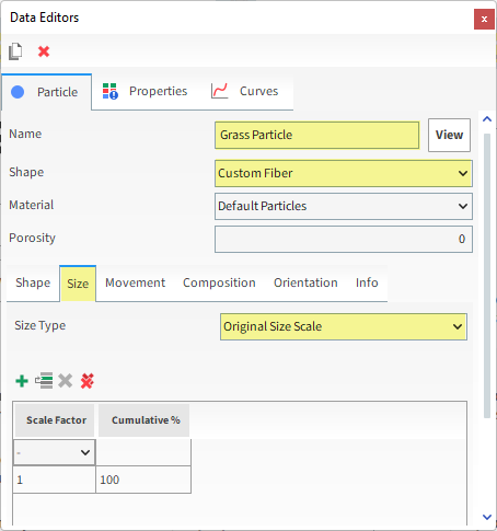
Create a new Particle.
From the main Particle tab, enter the Name, and then define the Shape as Custom Fiber.
From the Select file to import dialog, navigate to the geometry folder and open the grass.csv file.
From the Import File Info dialog, click OK.
From the Size sub-tab, set the Size Type.
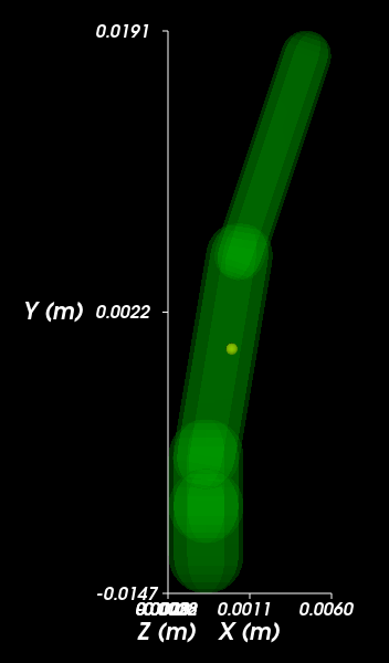
From the Data Editors panel, click the View button.
The particle shape representing a Grass Fiber is shown in a Particle Details window.
Because we designed this Custom Fiber shape in a .csv file, we don't have a copy of it we can use in a CAD program if, for any reason, we needed to.
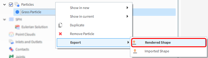
Luckily, Rocky enables us to export Particle shapes to .stl files. Let's try it:
From the Data panel, under Particles, right-click Grass Particle, point to Export and then click Rendered Shape.
From the Select output unit dialog, click OK.
From the Select target STL file dialog, choose a location and enter a File name for your file, and then click Save.
You now have an .stl copy of your grass Fiber shape.
For this tutorial, we want the grass Fibers to have a random orientation around the vertical axis:
From the Data Editors panel, select the Orientation sub-tab.
Enable the Random Angle checkbox and set the Half Angle (x,y,z).
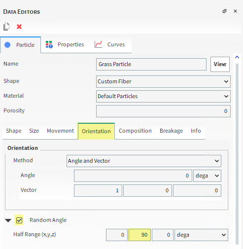
In this way, we have defined the Y-angle limit within which Rocky will randomly orient each individual particle within the Particle set.
For this tutorial, we want the grass Fiber to be both flexible in its movements and allow for the mower blades to cut (break) it on contact.
We will enable both these features by composing the Fiber of Multiple Elements.
By default, a Fiber is defined as a Single Element. This results in a rigid shape that cannot be broken.
In order to support both flexibility and breakage, Fibers must be composed of Multiple Elements, which divides each Segment into one or more Elements.
The number of Elements is (roughly) controlled by the Target Number of Elements number, and can be verified on the Info tab.
Flexibility and breakage both happen at the Joints that connect the Elements to each other.
For this tutorial, we want the number of Elements equal to the number of Segments making up the Fiber (4), so we will set the Target to a value less than or equal to this number.
From the Data Editors panel, select the Composition sub-tab, and then from the Composition list, select Multiple Elements.
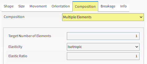
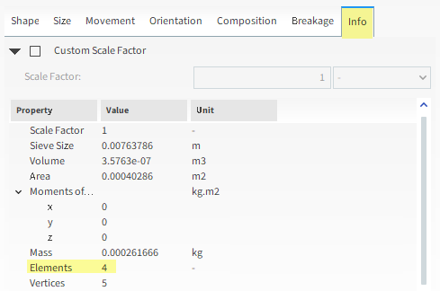
We can then verify the number of Elements Rocky will calculate on the Info tab. From the Info sub-tab, view the Elements value (as shown).
For Multi-Element particles, Rocky provides five model options for joint breakage:
Shear Stress Criterion
Griffith Surface Energy
Tensile Stress Criterion
Tensile or Shear Stress Criterion
von Mises Stress Criterion
Tip: Further information on these models can be found in the Rocky DEM Technical Manual.
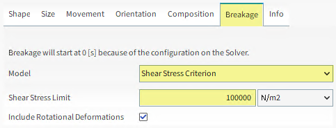
From the Data Editors panel, select the Breakage sub-tab, and then define the Model and Shear Stress Limit (as shown).
For this tutorial, we'll create a Particle Custom Inlet to exactly position the grass Fibers in a lawn-like pattern.
By previously defining the bottom Segment of our grass Fiber as frozen, we will ensure that the particles we position will stay stuck to the ground and upright, as if rooted.
If we had not taken this step, the grass Fibers would fall over soon after placement due to gravity and/or contacts with the mower.
To define the custom input, use the following information:
Step Data Entity Editors Location Parameter or Action Settings A Inlets and Outlets Create Particle Custom Inlet B Inputs ﹂Particle Custom Inlet <01>
Custom Input Particle Grass Particle ⯆ Load File grass_position.csv Motion Frame Translation ⯆
Because we are using multi-element Frozen Fibers, we can choose to attach them to a Motion Frame. Doing this enables the "frozen" part of the particles to move along with the assigned motions.
For this tutorial, we will assign the Translation Motion Frame, which will move the grass along with the ground towards the mower blades.
Important: When you attach a Motion Frame to a Particle Custom Inlet, the release property in the .csv file must be set to zero for all particles or omitted all together.
Under File Info, we can verify summarized info of the Properties that were defined inside the .csv we imported (as shown).
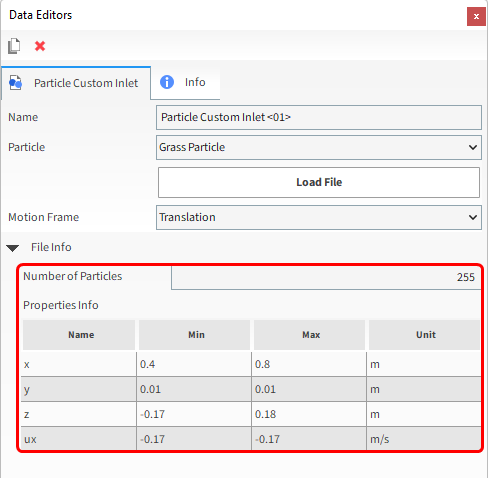
Note: The ux property set in the .csv file, which defines the initial velocity in the X-direction, was defined with the same velocity as our translation motion frame.
Doing this ensures all the Fiber's Segments start the simulation with the same velocity; otherwise, only the Frozen Segments would have the motion frame's velocity at 0s.
Use the information in the table that follows to define solver parameters and finish setting up your project.
Step Data Entity Editors Location Parameter or Action Settings A Solver Solver | Time Simulation Duration 3 [s] Output Settings | Time Interval 0.005 [s] Breakage | Start 0 [s] Breakage | Delay After Release 0 [s] Solver | General Simulation Target CPU ⯆
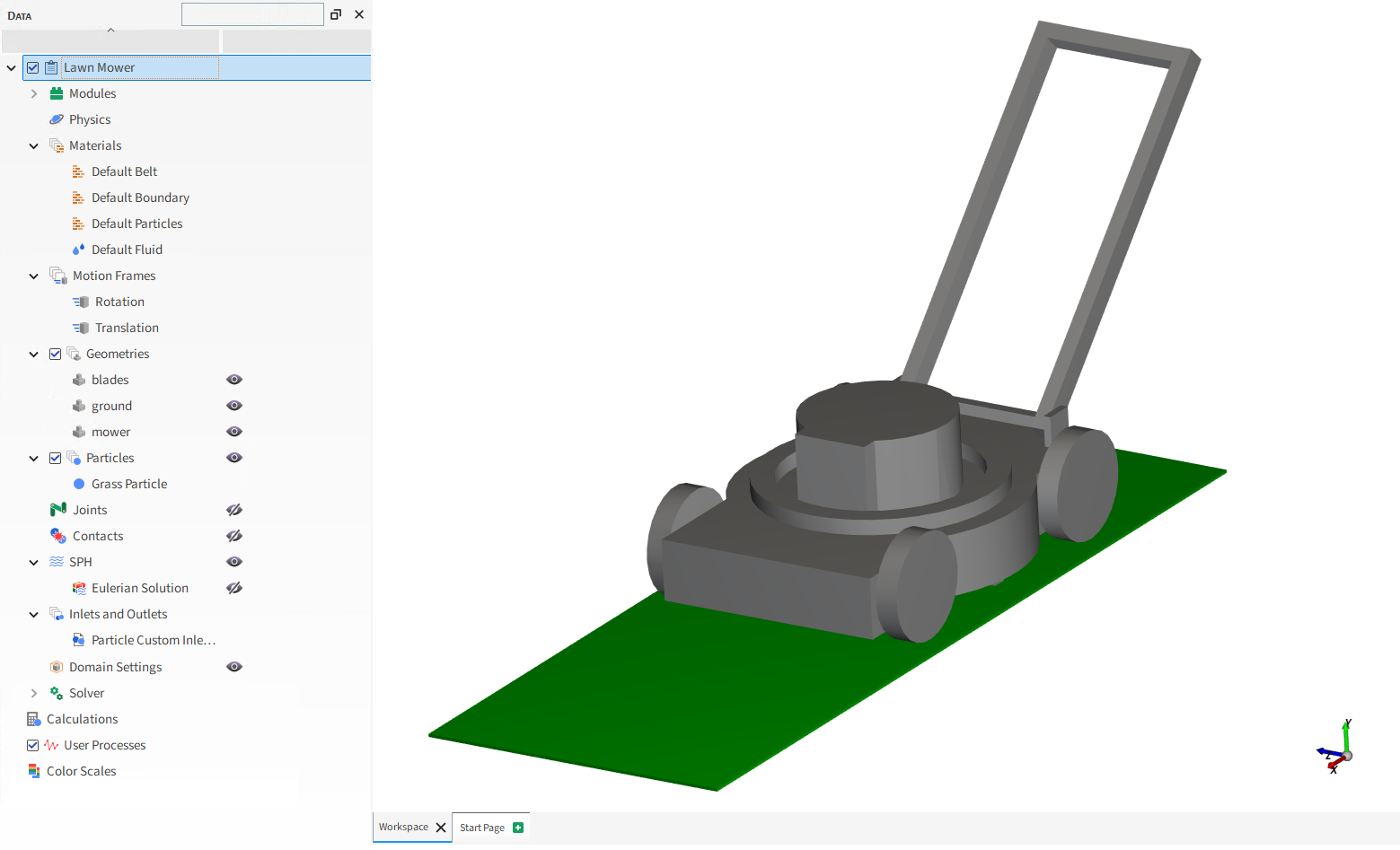
With a 3D View window opened, your Data panel and Workspace should look similar to the below image.
From the Solver entity, click Start.
The Simulation Summary screen appears (as shown), then processing begins.
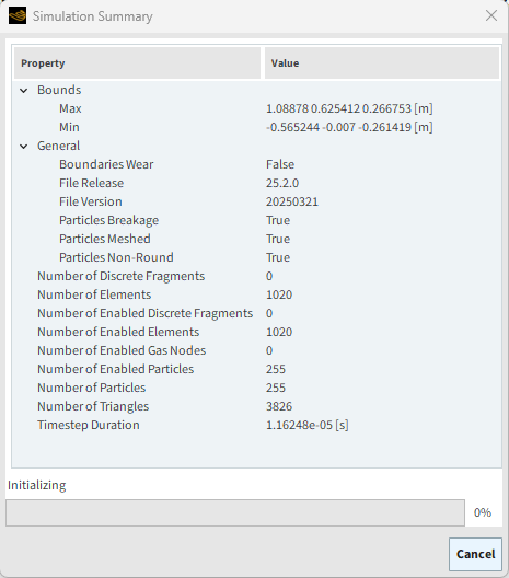
Tip: You can use the Auto Refresh checkbox to view in a 3D View window the results during processing.
This completes Part A of this tutorial, in which Rocky was used to set up and process a Lawn Mower simulation.
During this tutorial, it was possible to:
Understand how a Custom Fiber particle shape is composed.
Import a Custom Fiber particle shape that was defined with Frozen Segments.
Export a particle shape to an .stl file.
Set an appropriate Joint Breakage model for the Custom Fiber.
Assign a Motion Frame to a Particle Custom Inlet.
What's Next? If you completed this tutorial successfully, then you are ready to move on to Part B and post-process this project.
The purpose of this tutorial is to use the results from the simulation we set up and processed in Part A to analyze the performance of the Lawn Mower.
You will learn how to:
Use Particle Mass to view how a Fiber breaks
Calculate the Mower Blades' Power and Torque
Identify which Mower Blade regions are most susceptible to wear
And you will use these features:
Geometries Properties and Curves
Time Plots
Output Variables
Important: This ADVANCED tutorial contains fewer details, screenshots, and procedures than other Rocky tutorials.
An ADVANCED tutorial is designed for users who are more familiar with the Rocky user interface (UI), and already have a good understanding of the common setup and post-processing tasks.
If you do not already have this level of familiarity, it is recommended that you complete at least Tutorials 01 - 05 before beginning this one.
If you completed Part A of this tutorial, ensure that project is open in Rocky. (Part B will continue from where Part A left off.)
If you did not complete the project from Part A, do all of the following:
Download the
dem_tut22_files.zipfile here .Unzip
dem_tut22_files.zipto your working directory.Open Rocky 2025 R2.
Important: To make use of the Rocky project file provided, you must have Rocky 2025 R2 or later. If you have an earlier version of Rocky, please upgrade to the latest version, or complete Part A from scratch.
From the Rocky program, click the Open Project button, find the dem_tut22_files folder, then from the tutorial_22_A_pre-processing folder, open the tutorial_22_A_pre-processing.rocky file.
Process the simulation. (From the Solver entity, click the Start button.)
Use the information in the table below to see the effects of the blade geometry colliding with the grass Fibers.
Reminder: If you run into settings or procedures in these tables that you are not yet familiar with, please refer to the Rocky User Manual and/or other Tutorials (via the Introductory Tutorials and Advanced Tutorials) to find the detailed instructions you need.
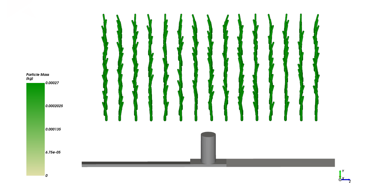
Step Item Location Parameter or Action Settings A Window (menu) Create a New 3D View B Particles Coloring Nodes (Enabled) Property Particle Mass ⯆
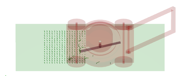
Initially, at 0 s into the simulation, each grass Fiber is whole (unbroken).
By moving the slider on the Time toolbar, you can observe how the mower blades cut the grass particles into fragments.
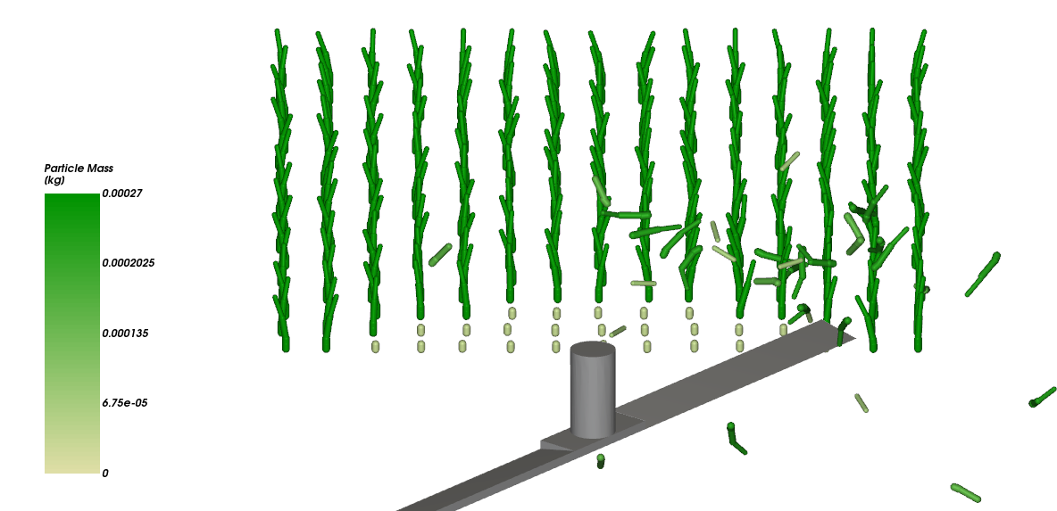
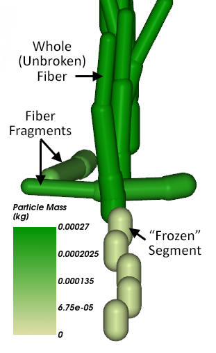
Note: For the Fibers that broke, only the frozen Segment of the Fiber remains upright.
In this tutorial we will estimate the Mower Blades torque according to:
 | (22–1) |
Where:
 is the torque (Nm)
  is the Power (W)
  is the angular frequency (Hz)
Use the information in the table below to create a Custom Curve for Torque.
Step Item Location Parameter or Action Settings A Geometries ﹂blades
Curves Add new custom curve (button) B Add new (dialog box) Name Torque Output Unit N.m Inputs | Power (Enabled) Inputs | Velocity : Rotational : Y (Enabled) C Custom Curves (dialog box) Expression A/(2*3.1416*B)
Note: For Step C, ensure the expression you enter represents:

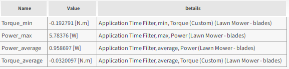
For this tutorial, we will assume that selecting the right size engine for our Lawn Mower requires us to know the following values:
Minimum Torque
Average Torque
Maximum Power
Average Power
We could create four separate Time plots and locate this information on each plot. However, this becomes more difficult when comparing values across multiple simulations.
An easier method is to use Output Variables, which distills a set of Property or Curve data into a single value in one easy-to-find location.
Let's use Output Variables to create the four single values we need for this analysis.
To create the Output Variables, do the following:
From the Tools menu, ensure that Expressions/Variables is enabled.
From the Data Editors panel, drag-and-drop the newly created Torque (Custom) Curve onto the Output tab. Repeat for the Power Curve.
From the Output tab, select the newly added Power entry, and then click the Edit
 button.
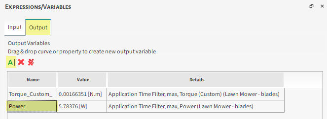
From the Edit Properties dialog, enter the Name, and then click OK.
Repeat for the Torque_Custom_ entry, entering the Name and defining the Operation on Curve.
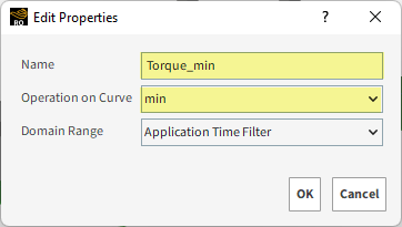
Note: As the blade spins counter-clockwise, the minimum Torque value will be the maximum absolute value.
Now we want the Average values.
From the Data Editors panel, drag-and-drop the Torque (Custom) Curve and the Power Curve onto the Output tab again.
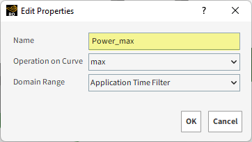
Select the newly added Power entry, and then click the Edit
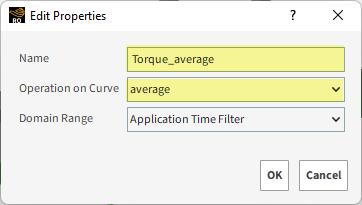
button. From the Edit Properties dialog, enter the Name, define the Operation on Curve (as shown), and then click OK.

Repeat for the Torque_Custom_ entry, entering the Name and defining the Operation on Curve.
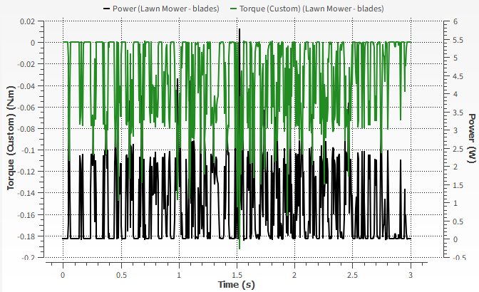
Press Ctrl+T to open a Time Plot.
From the Data Editors panel, drag-and-drop the newly created Torque (Custom) curve and the Power onto the Time Plot.
Now we have exactly the right Torque and Power values we need to choose an appropriate engine for our Lawn Mower.
In Rocky, you are able to compute the wear effects using surface wear modification.
The wear law used in that feature takes into account the shear work on the geometry surface to compute how it will wear down over time.
However, for the case we are studying in this tutorial, the surface modification of the mower blades would not be noticeable due to the short simulation time.
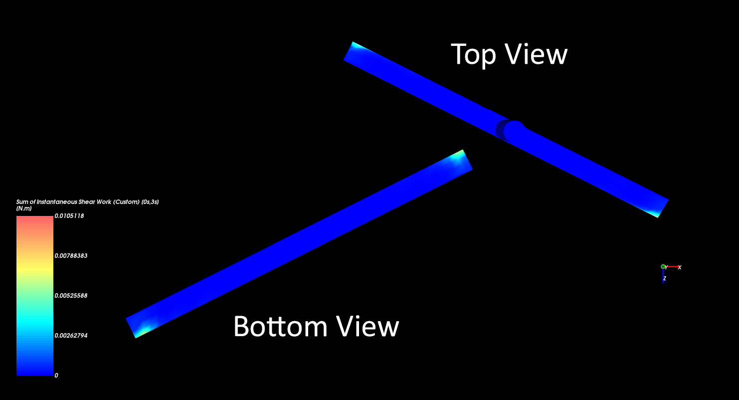
Instead, we can compute the total work done by the shear forces on each triangle surface and then verify which regions of the blades have the highest shear work.
You might recall that in Part A, we enabled the collection of Intensities data for Boundary Collision Statistics. We can use that data to perform the shear work analysis.
A good approximation of it would be:
 | (22–2) |
Where:
 (J) is the work
  (W/m2) is the Intensity : Shear, both of which act on the triangle,
 (m2) is the Area :
Cell, which is the area of the triangle
(m2) is the Area :
Cell, which is the area of the triangle  is the time (s)
 (s) is the time between 2 outputs, which is dictated by the Time Interval
Use the data in the following tables to add a new custom property that calculates the shear work in the blades:
Step Item Location Parameter or Action Settings A Geometries ﹂blades
Properties Add new custom property (button) B Add New (dialog box) Name Instantaneous Shear Work Output Unit J Inputs | Area : Cell (Enabled) Inputs | Intensity : Shear (Enabled) C Custom Property (dialog box) Expression A*B*OUTPUT_FREQUENCY D Geometries ﹂blades
Properties Add and edit time statistics properties (button) E Edit time statistics properties (dialog box) Add time statistics properties (button) F Add time statistics properties (dialog box) Start time 1 [s] Stop time 3 [s] Operations | Sum (Enabled) Properties | Instantaneous Shear Work (Custom) (Enabled) From the Properties tab, right-click the newly created Sum of Instantaneous Shear Work (Custom) property, point to 3D View, and then select Show in new 3D View.
From the Data panel, under Geometries, hide all but the blades component. Hide also the main Particles entity.
This completes Part B of this tutorial.
Rocky was used to post-process a simulation of a Lawn Mower cutting grass.
During this tutorial, it was possible to:
Use Particle Mass to view how a Fiber breaks.
Compute the mower blades' Torque by creating Custom Curves.
Use Output Variables to distill the mower blades' Torque and Power Curves into single, easy-to-locate values.
Compute total shear work done by the grass particles to the blades by creating Custom Properties and Time Statistics Properties.
What's Next? If you completed this tutorial successfully, then you are ready to move on to next tutorial.