SRS models, as described in Scale-Resolving Simulation (SRS) Models – Basic Formulations, serve the main purpose of dissipating the energy out of the turbulence spectrum at the limit of the grid resolution. The eddy viscosity is defined to provide the correct dissipation at the larger LES scales. This assumes that the numerical scheme is non-dissipative and that all dissipation results from the LES model. For this reason, one is required to select a numerical scheme in the LES region with low dissipation, relative to the dissipation provided by a subgrid LES model. Another strategy is to avoid the introduction of the LES (subgrid) eddy viscosity and provide all damping through the numerical scheme. This approach is called MILES (Monotone Integrated Large Eddy Simulation) (Boris et al., 1992 1). In Ansys CFD, the standard LES methodology is followed, whereby the dissipation is introduced by a LES eddy viscosity model and the numerical dissipation is kept at a low value.

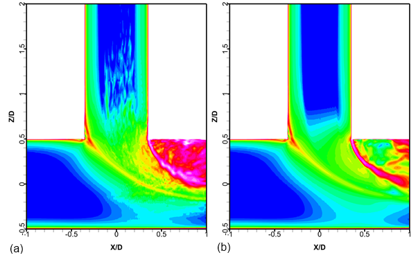
In order to achieve low numerical dissipation, you cannot use the standard numerical schemes for convection that were developed for the RANS equations (Second Order Upwind Schemes, or SOU), which are dissipative by nature. In contrast, LES is carried out using Central Difference (CD) schemes. In industrial simulations, second order schemes are typically employed, however, in complex geometries with non-ideal grids, CD methods are frequently unstable and produce unphysical wiggles (see Figure 12.60), which can eventually destroy the solution. To overcome this problem, variations of CD schemes have been developed with more dissipative character, but still much less dissipative than Upwind Schemes. An example is the Bounded Central Difference (BCD) scheme of Jasak et al., 1999 14.

Figure 12.60: Example of scheme oscillations in T-Junction flow shown by vorticity: (a) CD, (b) BCD

The CD scheme can be used successfully for (WM)LES of simple flows on optimal grids (typically hexahedral grids with low skew) such as channel or pipe flows. For more complex geometries, ELES allows the reduction of the LES domain to a limited region with high quality grids. Under such conditions, CD can be employed inside the LES portion of the grid, while using a standard upwind biased scheme for the RANS part of the domain.

For global models, like SAS or DDES/SDES/SBES, involving RANS and LES portions without a well-defined interface between them, most cases require the use of the BCD scheme, which can also handle both the RANS and LES domains with acceptable accuracy.

When using ELES in Ansys Fluent, one can also switch the numerical scheme between the RANS and the LES regions (see Cokljat et al., 2009 2) by hand.

In Ansys CFX, the default for the SAS and SBES models is a numerical scheme that switches explicitly between a second order upwind and the CD scheme, based on the state of the flow, using a switch proposed by Strelets, 2001 33. This switching scheme is relatively complex. It is advisable to apply the less complex BCD scheme that is also available in the software. In Ansys CFX there is an additional parameter for the BCD scheme that allows a continuous variation of the scheme from BCD to CD. The parameter is called CDS Bound. CDS Bound=1 applies only to BCD and CDS Bound=0 applies only to CD.

The spatial discretization of the convection terms of the turbulence model is second order by default. The use of second order upwind schemes can be beneficial for accurate RANS simulations. In case of numerical problems, it might be reasonable to try switching to the first order upwind scheme.

The selection of a specific gradient method is not of much relevance to SRSs on high quality hexahedral meshes. For skewed or polyhedral meshes, the Least Square Method (LSM) is recommended. For the SAS model one should use the LSM or the Green-Gauss Node Based (GGNB). The latter allows a slightly higher sensitivity to initial instabilities.

SRS can be relatively sensitive to the pressure interpolation. Validation studies have shown that the PRESTO scheme is more dissipative than the other options and should be avoided unless required for other reasons. For the validation studies, the standard pressure interpolation was typically used.

Time integration should be carried out with the second order backward Euler scheme. This has proven to have sufficient accuracy for a wide range of applications. For turbulence (and other positive) variables, use the Bounded Second Order Implicit Euler scheme (this must be selected in Ansys Fluent and is the default in Ansys CFX).

The time steps should be selected to achieve a Courant number of in the LES part of the domain. For complex geometries and grids with high stretching factors, the definition of the CFL number is not always very reliable (for example, if the flow passes through a region of highly stretched cells). In such situations, estimates can be built upon the physical dimensions of the shear layer to be resolved. If cubic cells are required for resolving a shear layer (say across a mixing layer of thickness ) and a certain CFL number is to be achieved, then a time step of

(12–33)

is required. Considering that is proportional to the RANS turbulent length scale (with a constant of order 1), this estimate may be further simplified to:

(12–34)

where . This simplified analysis means that the time step can be estimated on a pre-cursor RANS simulation.

You can also apply a more global estimate by assessing the through flow time, which is the time required by a fluid element to pass through the LES domain of length with velocity : . With an estimate of how many cells, , will be passed along this trajectory, one obtains .

There are several different settings for time advancement in Ansys Fluent. The first choice is between the Iterative (ITA) and the Non-Iterative Time Advancement (NITA). NITA should be checked for any new application as it can result in significant CPU savings. As a general guideline, NITA works well on high quality grids and for flows with limited additional physical coupling between the equations. Within NITA, the fractional step scheme is recommended; however, one must be very cautious and conservative with the assessment of the time step size. An attempt to perform a simulation with CFL>1 can lead to an incorrect solution. In addition, one should reduce residual tolerance for all equations to 0.0001.

For the ITA schemes (everything except NITA), the segregated solvers are typically faster than the coupled solver. The optimal choice is in most cases the SIMPLEC scheme. The default under-relaxation parameters for this scheme are set for steady-state simulations. For SRS model simulations, they should be changed to values as close as possible to 1 to improve iterative convergence. Typically, the number of inner iteration loops required with SIMPLEC depends on the complexity of the flow problem. The most critical quantity is the mass conservation. Mass residuals should decrease by at least one order of magnitude every time step. With high under-relaxation and good grid quality, good solutions can often be achieved even with only two inner loops.

The coupled solver is slower per iteration, but it can lead to more robust convergence, and for complex cases can be advantageous. For the coupled solver, one would typically also specify under-relaxation values of (or close to) 1. The number of inner loops is typically 2-5. In Ansys CFX, the coupled solver is used in all simulations.

For flows with additional physics (multiphase, combustion, and so on), the number of inner iterations per time step can increase for all solvers.

It is important to emphasize that the optimal under-relaxation factors and the optimal number of inner iterations is case-dependent. Some optimization might be required for achieving the most efficient results.