


The following topics are available concerning cyclically symmetric structure analysis:
Given a cyclically symmetric (periodic) structure, such as a fan wheel, a modal analysis can be performed for the entire structure by modelling only one sector of it. A proper base sector represents a pattern that, if repeated n times in cylindrical coordinate space, would yield the complete structure.

In a flat circular membrane, mode shapes are identified by harmonic indices. For more information, see the Cyclic Symmetry Analysis Guide.
Constraint relationships (equations) can be defined to relate the lower (θ = 0) and higher (θ = α, where α = sector angle) angle edges of the base sector to allow calculation of natural frequencies related to a given number of harmonic indices. The base sector is duplicated in the modal analysis to satisfy the required constraint relationships and to obtain nodal displacements. This technique was adapted from Dickens([149]).

Constraint equations relating the lower and higher angle edges of the two sectors are written:
 | (14–252) |
where:
 , ,  = calculated displacements on lower angle side of base and duplicated sectors
( = calculated displacements on lower angle side of base and duplicated sectors
( and and  , respectively) , respectively) |
 , , = displacements on higher angle side of base and duplicated sectors ( = displacements on higher angle side of base and duplicated sectors ( and and  , respectively) determined from constraint relationships , respectively) determined from constraint relationships |

|
 = sector angle = sector angle |
 = number of sectors in 360° = number of sectors in 360° |
Three basic steps in the procedure are briefly:
The CYCLIC command in /PREP7 automatically detects the cyclic symmetry model information, such as edge components, the number of sectors, the sector angles, and the corresponding cyclic coordinate system.
The CYCOPT command in /SOLU generates a duplicated sector and applies cyclic symmetry constraints (Equation 14–252) between the base and the duplicated sectors.
The /CYCEXPAND command in /POST1 expands a cyclically symmetry response by combining the base and the duplicated sectors results (Equation 14–253) to the entire structure.
The mode shape in each sector is obtained from the eigenvector solution. The displacement components (x, y, or z) at any node in sector n for harmonic index k, in the full structure is given by:
where:
 | (14–253) |
 = sector number, varies from 1 to = sector number, varies from 1 to 
|
 = mode number = mode number |
 = base sector displacement = base sector displacement |
 = duplicate sector displacement = duplicate sector displacement |
 = arbitrary phase angle = arbitrary phase angle |
If the mode shapes are normalized to the mass matrix in the mode analysis (via
Nrmkey on the MODOPT command), the normalized
displacement components in the full structure are given
by:
 | (14–254) |
If the mode shapes are normalized using the maximum value of the mode
(Nrmkey = ON in the MODOPT command), the
normalization equation is:
 | (14–255) |
where
 = mode number = mode number |
 = DOF number = DOF number |
The complete procedure addressing static, modal, and prestressed modal analyses of cyclically symmetric structures is contained in the Cyclic Symmetry Analysis Guide.
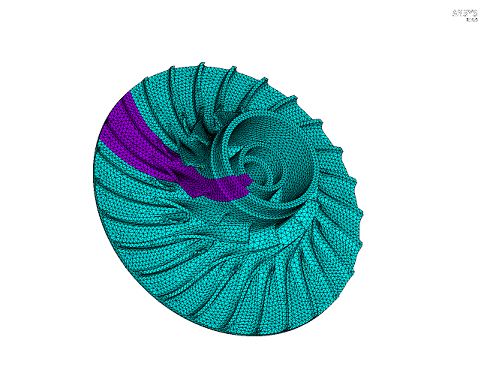
A bladed disk (axial or centrifugal) is cyclically symmetric about its fundamental sector, as shown in Figure 14.16: Full Model with the Cyclic-Symmetric Sector Highlighted. These bladed disks are typically excited by rotationally symmetric excitations which produce forced vibrations.
The equation of motion for harmonically-varying forced response is:
 | (14–256) |
where:
 = stiffness matrix of the bladed disk = stiffness matrix of the bladed disk |
 = mass matrix of the bladed disk = mass matrix of the bladed disk |
 = load vector = load vector |
 = displacement vector = displacement vector |
 = forcing frequency, input on the CYCFREQ command = forcing frequency, input on the CYCFREQ command |
The superscript  implies the matrices refer to the entire 360° system. Damping is ignored
in this equation and is discussed in Damping.
implies the matrices refer to the entire 360° system. Damping is ignored
in this equation and is discussed in Damping.
Equation 14–256 can be transferred into modal space by:
 | (14–257) |
where:
 = the set eigenvectors of the full system = the set eigenvectors of the full system |
 = the vector of modal coordinates = the vector of modal coordinates |
Substituting this into Equation 14–256 and pre-multiplying by
 yields the forced response equation in terms of modal coordinates:
 | (14–258) |
where:
 = the diagonal matrix for the system natural frequencies squared = the diagonal matrix for the system natural frequencies squared |
 = the identity matrix = the identity matrix |
The number of eigenvectors (modes) used in Equation 14–258 is much less than the total number of degrees of freedom, so that Equation 14–258 is significantly smaller system than Equation 14–256.
A cyclically-symmetric structure has the following transformation from cyclic coordinates to physical coordinates:
 | (14–259) |
where:
 = cyclic (or harmonic) coordinates for harmonic index = cyclic (or harmonic) coordinates for harmonic index 
|
 = real-valued Fourier matrix = real-valued Fourier matrix |
 denotes the Kronecker product denotes the Kronecker product |
The system eigenvectors can also be expressed in terms of their harmonics:
 | (14–260) |
where:
 = the real-valued cyclic modes corresponding to harmonic = the real-valued cyclic modes corresponding to harmonic
|
 = a pseudo-block diagonal matrix. A block is 1×1 for = a pseudo-block diagonal matrix. A block is 1×1 for  = 0 and = 0 and  if if  is even, and 2×2 otherwise. is even, and 2×2 otherwise.  is the number of sectors (CYCLIC). is the number of sectors (CYCLIC). |
Substituting Equation 14–260 into Equation 14–258 gives the frequency response equation in cyclic coordinates:
 | (14–261) |
where the modal load  is:
is:
 | (14–262) |
The Fourier transformation expression:
 | (14–263) |
appears in Equation 14–260 and Equation 14–262
(transposed), where  are the harmonic modes.
  has the structure:
 | (14–264) |
The harmonics  (0 <
(0 <  <
<  ) appear as 2×2 sub-blocks, each column being one of the repeated modes
and the rows corresponding to the real and imaginary (base and duplicate sector) solutions. The
first mode in a pair is denoted with subscript
) appear as 2×2 sub-blocks, each column being one of the repeated modes
and the rows corresponding to the real and imaginary (base and duplicate sector) solutions. The
first mode in a pair is denoted with subscript  and the second mode in the pair is denoted with subscript
  .
.
The real and imaginary terms of each double mode are related and obey the following:
 | (14–265) |
where  = 1 if the mode shapes
  and
and  have the same sign, otherwise
  = -1. Likewise:
 | (14–266) |
where  . This property leads to the .MODE file needing to only
contain the real (base) sector degrees of freedom for each mode shape. Likewise, the stresses
and strains for the expanded modes on the .RST file only contain the
results for the base elements (and not the duplicate elements).
. This property leads to the .MODE file needing to only
contain the real (base) sector degrees of freedom for each mode shape. Likewise, the stresses
and strains for the expanded modes on the .RST file only contain the
results for the base elements (and not the duplicate elements).
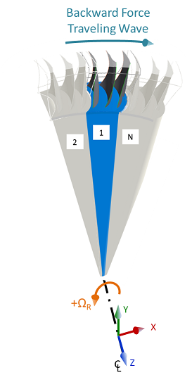
The forcing function is assumed to be time harmonic as well as spatially harmonic in the circumferential direction. The force on any sector n can then be related to the force on the base sector by only a phase shift:
 | (14–267) |
where:
 = complex load vector on the base sector = complex load vector on the base sector |
 = phase of excitation (inter-blade phase angle, IBPA) = phase of excitation (inter-blade phase angle, IBPA) |
 = sector number = sector number |
 = engine order (EO) excitation (CYCFREQ) = engine order (EO) excitation (CYCFREQ) |
 = number of sectors = number of sectors |
Equation 14–267 defines the distribution of force over the blades using the
blade numbering convention shown in Figure 14.17: Forcing Sign and Numbering Convention. With this
convention, blade 2 leads blade 1 by the inter-blade phase angle  ; it is subjected to the force first and blade 1 is subjected to the same force
after a rotation of
; it is subjected to the force first and blade 1 is subjected to the same force
after a rotation of  radians. The forcing wave travels in the direction shown in Figure 14.17: Forcing Sign and Numbering Convention, which is a backward traveling wave with respect to the
rotation
radians. The forcing wave travels in the direction shown in Figure 14.17: Forcing Sign and Numbering Convention, which is a backward traveling wave with respect to the
rotation  (OMEGA or CMOMEGA).
Equation 14–262 can be written as the sum of each sector, if only blade loads are considered:
 | (14–268) |
where:
 = the = the  row of the Fourier matrix row of the Fourier matrix 
|
 = force on blade = force on blade 
|
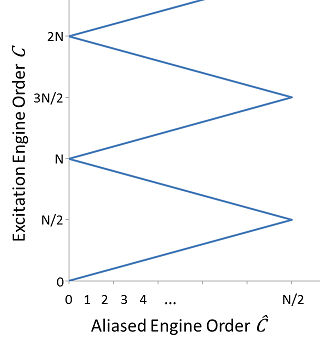
While the engine order can take any integer value, a given engine order
 will only excite a certain harmonic index. This aliased engine order
 is determined from the input engine order (for example, the
number of preceding stators) as outlined in the following table:
is determined from the input engine order (for example, the
number of preceding stators) as outlined in the following table:
Table 14.2: Aliased Engine Order (Excited Harmonic Index)
Engine Order 
| Aliased Engine Order 
| |
|---|---|---|
 Even Even |
 Odd Odd | |

|

|

|

|

|

|

|

|

|

|

|

|
| … | … | … |
This leads to the well-known zigzag diagram in Figure 14.18: Zigzag Diagram for an Even Number of Sectors. The positive slopes (positive aliased engine order) are backward traveling waves and the negative slopes are forward traveling.
Due to the orthogonality of the engine order phasing with the sine and cosine terms of the
Fourier matrix  , only the harmonic indices
  =
=  of
of
 are non-zero.
The sign of  is determined as follows:
If the aliased engine order is on a negative slope of Figure 14.18: Zigzag Diagram for an Even Number of Sectors, it is assigned a negative value.
If the rotation is opposite that illustrated in Figure 14.17: Forcing Sign and Numbering Convention, in other words a negative
 in the cyclic coordinate system, the value from the first step is
negated.
in the cyclic coordinate system, the value from the first step is
negated.If the engine order was input as a negative value, the value after the second step is negated again.
This process ensures that the force is correctly applied to the blades via Equation 14–262, while respecting the blade numbering, rotation direction, and the relationship between engine order and nodal diameter.
Returning to the harmonic equation of motion, Equation 14–261, the force is assumed to be harmonic and of the form:
 | (14–269) |
The excitation frequency  , and the corresponding frequency sweep range
  (HARFRQ) is typically related to the rotor speed by:
 | (14–270) |
The maximum response will occur when this excitation frequency crosses a natural frequency
of that nodal diameter, for instance when  .
.
Damping may be included in the following forms:


The damping matrix in cyclic modal coordinates is
 | (14–271) |
where
 = diagonal matrix of system frequencies = diagonal matrix of system frequencies |
 = diagonal matrix of modal damping terms = diagonal matrix of modal damping terms 
|
It is also possible to apply aerodamping as a part of aerodynamic coupling, which is addressed in the following section.
Interblade aerodynamic coupling can be introduced assuming a first
order dependence on the blade motion by inserting an additional matrix  (input using CYCFREQ,AERO) into the frequency response
equation of motion for the whole system. First consider the introduction of the aero matrix in
physical coordinates:
(input using CYCFREQ,AERO) into the frequency response
equation of motion for the whole system. First consider the introduction of the aero matrix in
physical coordinates:
 | (14–272) |
where non-aero damping terms are dropped for conciseness. This equation can be transformed into modal coordinates using Equation 14–257.
 | (14–273) |
The aerodynamic coupling matrix in physical coordinates
 can be written in cyclic cantilevered blade coordinates (see He et. al. [431]):
 | (14–274) |
where  is the complex-valued Fourier matrix and
  is a matrix of cantilevered blade modes. The resulting matrix
  is in general complex since the coupling is not in phase with the motion, but
it is presumed to be cyclically symmetric and therefore block diagonal:
is in general complex since the coupling is not in phase with the motion, but
it is presumed to be cyclically symmetric and therefore block diagonal:
 | (14–275) |
Note that a sub-block  corresponds to the interblade phase angle
  , where
  . It is common for CFD and other codes to compute the aerodynamic coefficients
that are compatible with this matrix. Each block
. It is common for CFD and other codes to compute the aerodynamic coefficients
that are compatible with this matrix. Each block  is made up of coefficients
  , that capture the coupling between mode i and the force computed using mode j
in the direction of the surface normal. These values can be obtained using the following area
integral:
, that capture the coupling between mode i and the force computed using mode j
in the direction of the surface normal. These values can be obtained using the following area
integral:
 | (14–276) |
where  is the surface normal and
  is the area.
The aerodynamic term in Equation 14–273 can
be rewritten by assuming that the blade portion ( ) of the system modes can be represented by a linear combination of cantilevered
blade modes:
) of the system modes can be represented by a linear combination of cantilevered
blade modes:
 | (14–277) |
The aero term becomes:
 | (14–278) |
Rearranging Equation 14–274 and substituting into Equation 14–278, it can be seen that the aero term is:
 | (14–279) |
Once the vector of modal coordinates  is obtained for a given excitation frequency
  , we can expand back to the physical solution quantities for the entire bladed
disk. The displacements of sector
, we can expand back to the physical solution quantities for the entire bladed
disk. The displacements of sector  are determined by:
 | (14–280) |
Stresses and strains can be similarly evaluated by using the stress and strain mode shapes
for
 .
.
The program employs the CMS-based Component Mode Mistuning (CMM) methodology (see Lim et. al. [425]) for small stiffness mistuning. This methodology is well suited not only to the simulation of bladed disks, but also to integrally bladed rotors and impellers where coupled disk-blade motion is important. From a tuned response of the nominal geometry, mistuning parameters are introduced into the component modes which are projected onto the system modes, yielding a compact set of equations for the harmonic frequency response of the system. This methodology builds on the theory discussed in Mode-Superposition Harmonic Analysis, and shares the basic core equations, damping, forcing, and coordinate transformations.
Stiffness mistuning can be characterized as a variation of the nominal stiffness of a system. Referring to Equation 14–256, the stiffness matrix can be written as:
 | (14–281) |
where the subscript o indicates the nominal values and  indicates deviations from the nominal. If the mistuning is assumed to be in
the blade only, we can assume proportional mistuning:
indicates deviations from the nominal. If the mistuning is assumed to be in
the blade only, we can assume proportional mistuning:
 | (14–282) |
where  is the nominal stiffness matrix for a blade and
  is the stiffness mistuning deviation for blade n. For a prestressed
analysis,
is the stiffness mistuning deviation for blade n. For a prestressed
analysis,  will include any prestress effects. This may alternatively be
considered as deviation in Young's modulus only in the case where there are no prestress
effects.
will include any prestress effects. This may alternatively be
considered as deviation in Young's modulus only in the case where there are no prestress
effects.  denotes a block diagonal matrix.
Mode-superposition is used to project the equation of motion onto an appropriate basis and reducing it to a smaller set of degrees of freedom. In contrast to typical mode-superposition techniques where the equation of motion is projected onto the modes computed from its own system (in this case, modes of the mistuned system), the program projects onto tuned system modes. Following the same reasoning as in Transform to Modal Coordinates, the forced response equation in tuned-system modal coordinates is:
 | (14–283) |
where  is the diagonal matrix of the system natural frequencies squared and [I] is
the identity matrix. The left superscript
is the diagonal matrix of the system natural frequencies squared and [I] is
the identity matrix. The left superscript  indicates that only the blade DOFs are used from the eigenvectors.
Substituting Equation 14–282 into Equation 14–283 and recognizing that the global triple product can be replaced with a local sum per sector yields:
 | (14–284) |
where N is the number of sectors.
The blade matrix  in Equation 14–284 can be approximated by applying
the fixed-interface Craig-Bampton (C-B) transformation:
in Equation 14–284 can be approximated by applying
the fixed-interface Craig-Bampton (C-B) transformation:
 | (14–285) |
where  are the generalized C-B coordinates (modal participation factors), and the
transformation
are the generalized C-B coordinates (modal participation factors), and the
transformation  is given by:
 | (14–286) |
 are the set of blade modes derived from assuming the blade-disk interface is
fixed (and any shroud interfaces as well), and
are the set of blade modes derived from assuming the blade-disk interface is
fixed (and any shroud interfaces as well), and  are the static shapes:
 | (14–287) |
where the subscripts  and
and  indicate the partition into internal and boundary (interface) DOFs of the
blade. Note that b corresponds to master DOFs and
indicate the partition into internal and boundary (interface) DOFs of the
blade. Note that b corresponds to master DOFs and  corresponds to all remaining DOFs in the substructure as defined in Component Mode Synthesis (CMS). The boundary DOFs and the elements defining the blade matrices are both
input on CYCFREQ,BLADE.
corresponds to all remaining DOFs in the substructure as defined in Component Mode Synthesis (CMS). The boundary DOFs and the elements defining the blade matrices are both
input on CYCFREQ,BLADE.
Applying this transformation to the blade stiffness yields:
 | (14–288) |
The number of blade modes is typically small leading to  being a much smaller matrix than
  .
.
Note that this is the typical Component Mode Synthesis (CMS) substructure generation analysis for the blade.
Projecting the Craig-Bampton coordinates  onto the system modes for a sector via:
 | (14–289) |
and substituting into Equation 14–284 yields for the blade stiffness term:
 | (14–290) |
The CMM approach to mistuning allows for the use of cyclic quantities
within the reduced equations of motion. The Craig-Bampton coordinates or modal participation
factors for the  sector can be expressed in cyclic coordinates using the same transformation as
in Equation 14–259:
sector can be expressed in cyclic coordinates using the same transformation as
in Equation 14–259:
 | (14–291) |
where
 is the
  row of
 . Substituting Equation 14–290 into Equation 14–284 and using Equation 14–291
and Equation 14–260 we arrive at:
. Substituting Equation 14–290 into Equation 14–284 and using Equation 14–291
and Equation 14–260 we arrive at:
 | (14–292) |
where the modal load  is:
is:
 | (14–293) |
Rewriting Equation 14–285 in cyclic coordinates:
 | (14–294) |
and segregating  into
its parts yields:
into
its parts yields:
 | (14–295) |
From the definition of [T] in Equation 14–286, it is clear that:
 | (14–296) |
where  are the system modes at the blade
interface points.
are the system modes at the blade
interface points.
Premultiplying Equation 14–294 by
 and using orthogonality of the modes, we can solve for
  :
:
 | (14–297) |
where  and
and  are the blade natural frequencies squared and mode shapes from the
Craig-Bampton transformation.
are the blade natural frequencies squared and mode shapes from the
Craig-Bampton transformation.
The stiffness parameter  (input on CYCFREQ,MIST) is handled as follows.
The stiffness mistuning parameter  represents the deviation of Young’s modulus
of each blade from its nominal value:
represents the deviation of Young’s modulus
of each blade from its nominal value:
 | (14–298) |
This leads to a modification of the blade’s natural frequencies by a common factor. In order to modify each natural frequency independently, a frequency-dependent mistuning parameter is introduced:
 | (14–299) |
where  is the
  nominal frequency of blade
  and
and  is the
 mistuned frequency of blade
  . Note that if
  is constant for all frequencies, then
  , that is, when all frequencies are modified by the same ratio that is
identical to the modified Young’s modulus.
, that is, when all frequencies are modified by the same ratio that is
identical to the modified Young’s modulus.
The application of the effective stiffness mistuning parameter  is as follows. The
nominal Craig-Bampton reduced stiffness matrix has the following form,
after applying the transformation in Equation 14–286:
is as follows. The
nominal Craig-Bampton reduced stiffness matrix has the following form,
after applying the transformation in Equation 14–286:
 | (14–300) |
Defining the average frequency mistuning for a blade as:
 | (14–301) |
where  is the number of blade frequencies, we can define the stiffness mistuning
as:
is the number of blade frequencies, we can define the stiffness mistuning
as:
 | (14–302) |
The constraint modes are modified by the average frequency mistuning, and the frequencies themselves are modified by the frequency-dependent input values.
The cyclically symmetric solution sequences consist of three basic
steps. The first step transforms applied loads to cyclically symmetric components using finite
Fourier theory and enforces cyclic symmetry constraint equations (see Equation 14–252) for each harmonic index (nodal diameter)
( = 0, 1, . . .,
  ).
).
Any applied load on the full 360° model is treated through a
Fourier transformation process and applied on to the cyclic sector. For each value of harmonic
index,  , the procedure solves the corresponding linear equation. The responses in each
of the harmonic indices are calculated as separate load steps at the solution stage. The
responses are expanded via the Fourier expansion (Equation 14–253). They are then combined to get the complete
response of the full structure in postprocessing.
, the procedure solves the corresponding linear equation. The responses in each
of the harmonic indices are calculated as separate load steps at the solution stage. The
responses are expanded via the Fourier expansion (Equation 14–253). They are then combined to get the complete
response of the full structure in postprocessing.
The Fourier transformation from physical components,  , to the different harmonic index components,
  , is given by the following:
Harmonic Index,  = 0 (symmetric mode):
 | (14–303) |
Harmonic Index, 0 <  <
<  (degenerate mode)


For  even only, Harmonic Index,
  (antisymmetric mode):
 | (14–306) |
where:
 = any physical component, such as displacements, forces, pressure loads,
temperatures, and inertial loads = any physical component, such as displacements, forces, pressure loads,
temperatures, and inertial loads |
 = cyclically symmetric component = cyclically symmetric component |
The transformation to physical components,  , from the cyclic symmetry,
  , components is recovered by the following equation:
 | (14–307) |
The last term,  , exists only for
  even.
even.