


User-programmable features (UPFs) are available with coupled-field elements PLANE222, PLANE223, SOLID225, SOLID226, and SOLID227. Coupled-field UPFs enable you to customize element characteristics, material models, loads, constitutive equations, element matrices and load vectors, and output items. The UPFs give you access to all the applicable element results at any location within the element, making it easier to program nonlinearities. The coupled-field UPFs are integrated into the element standard workflow, so you can customize the element property of interest without writing a user element or a user material model from scratch. For your convenience, there are several utility functions available to help you access element results and other element information.
The following topics are available:
- 2.4.1. Activating Programmable Features for Supported Analysis Types
- 2.4.2. Files on the Distribution Media
- 2.4.3. Coding Coupled-field UPFs
- 2.4.4. Example: User implementation of stress- and electro-migration analysis
- 2.4.5. Example: User Implementation of Thermoplastic Heating
- 2.4.6. Example: User-defined Diffusing Substance Generation Rate
- 2.4.7. Example: User-defined Damping
- 2.4.8. Example: User-defined Diffusivity
User-programmable capabilities are available with coupled-field elements PLANE222, PLANE223, SOLID225, SOLID226, and SOLID227 for the following coupled-diffusion analyses:
Structural-diffusion (KEYOPT(1) = 100001)
Thermal-diffusion (KEYOPT(1) = 100010)
Electric-diffusion (KEYOPT(1) = 100100)
Thermal-Electric-Diffusion (KEYOPT(1) = 100110)
Structural-thermal-diffusion (KEYOPT(1) = 100011)
Structural-electric-diffusion (KEYOPT(1) = 100101)
Structural-thermal-electric-diffusion (KEYOPT(1) = 100111)
To activate user-programmable features (UPFs), set KEYOPT(12) = 1 on the coupled-field elements used in any of the above analyses. Activating UPFs enables you to define or modify the element material properties, loads, constitutive equations, element matrices and load vectors, as well as element results. Multiple functions and subroutines are available to provide you with convenient access to the element and solution information.
The UserProcedures.F file contains the source code for the routines that provide an interface to the coupled-field element code and allow you to add code to customize its behavior. This file can be found on the distribution medium along with other user routines (see Studying the Mechanical APDL User Routines).
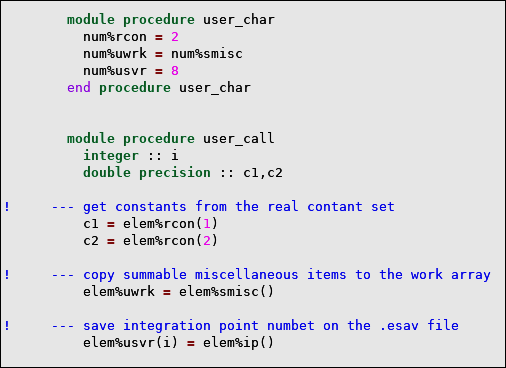
The coupled-field UPF code is implemented as a Fortran submodule programming unit [1] that contains two procedures, user_char and user_call. You add code in these procedures as follows:
user_charAdd code to modify element characteristics, including number of work variables, saved variables, SMISC and NMISC items, element matrix symmetry, and element nonlinearity as detailed in Modifying the Coupled-field Element Characteristics (
user_char).user_callAdd code to modify element calculations, such as material properties, loads, element matrices, and load vectors using the utility functions described in Customizing Element Calculations (
user_call).
Both procedures must be present to successfully compile and link UserProcedures.F. The following figure shows the procedures user_char and user_call. Note that there is no default code in the procedures.
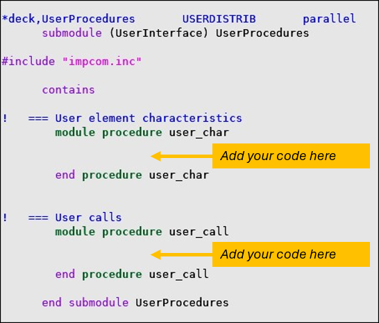
You can alter the submodule name (UserProcedures in Figure 2.1: UserProcedures.F file ) but not the module name (UserInterface).
Note that when you compile UserProcedures.F, the UPF tools automatically accesses the ancestor module file userinterface.mod. You do not modify this file, but it must be present at the following path:
Linux
/ansys_inc/v252/ansys/customize/include/userinterface.mod
Windows
Program Files\ANSYS Inc\V252\ansys\customize\include\userinterface.mod
References
A useful reference on modern FORTRAN is:
The element code makes additional calls to the two subroutines
user_char and user_call when
user-programmable features (UPFs) for a coupled-field analysis are enabled
(KEYOPT(12) = 1). These calls enable you to customize element characteristics and
element calculations by modifying the user_char and
user_call procedures, respectively.
The next sections describe how
user_char and user_call procedures
interact with the standard coupled-field element behavior. The following
abbreviations are used in the description of input and output
arguments:
| int – integer | ar – array | |
| dp – double precision | in – input | |
| log – logical | out – output | |
| sc – scalar | none – no argument |
Element characteristics are programmed as an array of integer numbers (approximately 200)
that define the element and control its behavior. The
user_char procedure enables you to reset some of these
element characteristics. All other characteristics default automatically.
user_char is called once from the element routine that
sets these default characteristics.
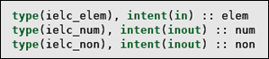
The information about element characteristics is passed to user_char
in the form of three data structures: num,
non, and elem as shown in Figure 2.3: user_char Procedure
Interface. This
interface information resides in the userInterface.mod file
and is not replicated in the procedure body in
UserProcedures.F.
A brief description of user_char arguments is given in
the following table.
Table 2.1: user_char Procedure Arguments
| Name | Type | Content |
|---|---|---|
| num | ielc_num | sizes of element data arrays |
| non | ielc_non | element formulations |
| elem | ielc_elem | element definitions |
user_char procedure: num
structure
Components of the num structure can be used to customize some of the element characteristics as follows:
num%
itemwhere:
itemname of the characteristics.
Table 2.2: num Structure Components
item | Description | Type |
| rcon | number of real constants | int sc |
| smisc | number of summable miscellaneous items | |
| nmisc | number of non-summable miscellaneous items | |
| usvr | number of user saved variables | |
| uwrk | number of user variables |
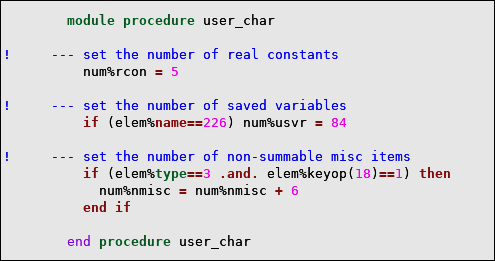
For example,
num%rcon = 5
sets the number of real constants to 5, and
num%smisc = num%smisc + 2
adds 2 to the default number of summable miscellaneous. Note that you can only increment the number of real constants (num%rcon), the number of summable (num%smisc), or non-summable (num%nmisc) variables. In other words, the custom number of real constants or miscellaneous variables cannot not be less than the default number of real constants/miscellaneous variables listed in element descriptions (Element Reference).
user_char procedure: non
structure
Components of the non structure can be used to set the characteristics that control the element formulation:
non%
itemwhere:
itemname of the element property.
Table 2.3: non Structure Components
item | Description | Type | Value |
| sym | element matrix | int sc |
0 – symmetric 1 – unsymmetric 2 – symmetric, but may become unsymmetric due to certain material models |
| lin | element linearity |
0 – linear element 1 – nonlinear element |
For example,
non%sym = 1
sets the element matrix to nonsymmetric.
user_char procedure: elem
structure
When modifying the above element characteristics, you can access (use in read-only mode) the following components of the elem structure:
elem%
itemwhere:
itemname of the characteristics.
Table 2.4: elem Structure Components
item | Decription | Type |
|---|---|---|
| type | element type | int sc |
| name | element name | |
| keyop(kyop) | element keyoption (kyop = 1 from 18) |
The following example illustrates customization of the element characteristics using the
user_char procedure.
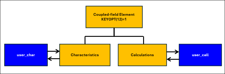
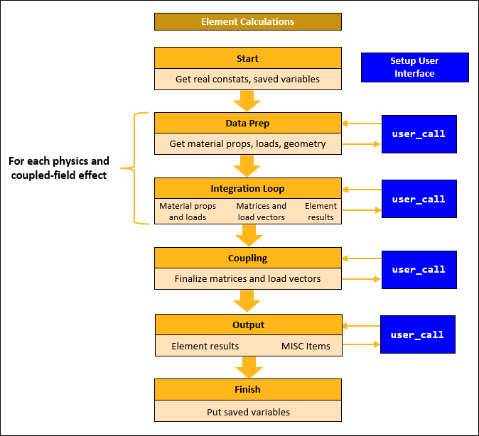
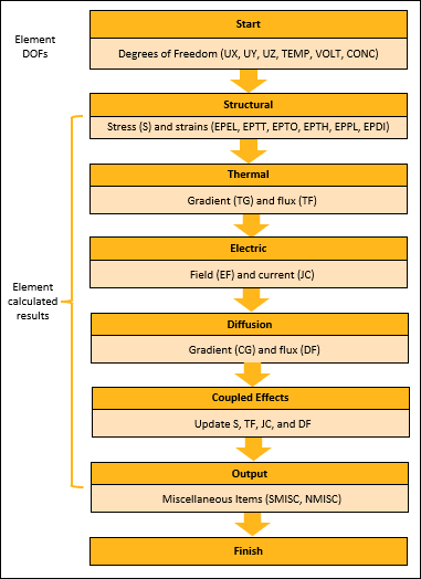
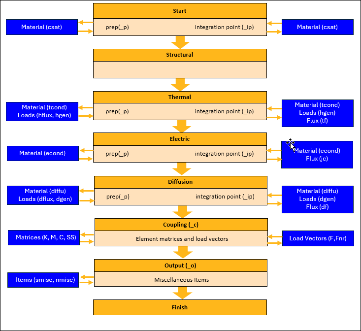
Typical element calculations have four distinct phases: data preparation, integration point calculations, coupled-field calculation, and the output of element results (Figure 2.4: Element Calculation Workflow).
Data preparation — Material properties and element loads are first evaluated during the data preparation stage.
Integration point calculations — Material properties, loads, and element results are then evaluated at each integration point using available solution information, for example, element results from the previous iteration. Element matrices and load vectors are formed in the same integration loop using numerical integration over the element volume.
Note: Data preparation and numerical integration are performed for each physics and coupled-field effect.
Coupled-field calculations — Following the numerical integration, element matrices and load vectors are finalized to include all the necessary physics and coupled-field effects.
Output of element results — During the output stage, all calculated element quantities are processed, and element results are written to the result file.
The user_call procedure is called multiple times during these four stages of element calculations. You can use user_call to:
Customize the evaluation of material properties and loads at both the data preparation and integration point stage.
Modify the constitutive relations at the integration point stage.
Modify the element matrices and load vectors at the coupling level of element calculations.
Modify the element miscellaneous items in the output phase of element calculations.
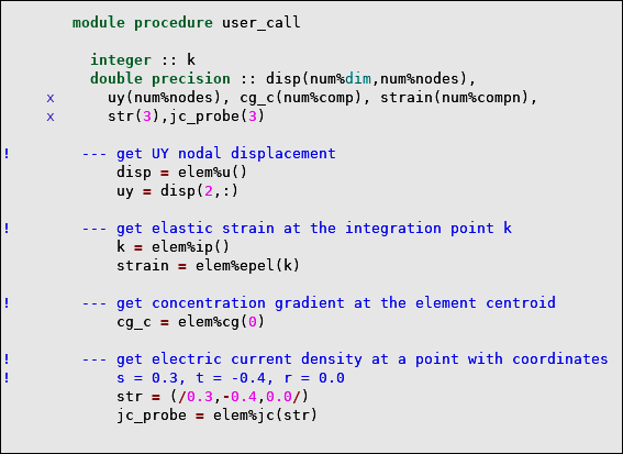
The information about the coupled-field element that can be passed to and used in
user_call is in the form of four structures: num, elem, solu, and scope. The
interface information (Figure 2.5: user_call Procedure Interface) resides in the
userInterface.mod file and is not replicated in the
procedure body.
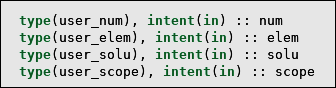
A brief description of user_call arguments is given in
the following table.
Table 2.5: user_call Procedure Arguments
| Name | Type | Content |
|---|---|---|
| num | user_num | Numbers that characterize element entities. |
| elem | user_elem | Components and procedures to access element characteristics, nodes, coordinates,
shape functions, and results.
Procedures to perform operations on element results and print these results. Procedures to define or modify material properties, loads, constitutive equations, element matrices and load vectors, and output quantities |
| solu | user_solu | Solution settings and data to control element calculations. |
| scope | user_scope | Parameters to define the scope of element calculations. |
The components and type-bound procedures of these structures are described in detail below.
user_call procedure: num
structure (numerical element properties)
The num structure consists
of frequently used numerical element properties. All the components of this
structure are integer scalar parameters. Use these parameters to define the
sizes of variables in the user_call procedure or control
do-loop and if-constructs:
num%
itemwhere:
itemname of element property.
Table 2.6: Numerical Element Properties
item | Description | Type |
| dim | element dimensionality (2 or 3) | int sc |
| nodes | number of element nodes | |
| cnodes | number of element corner nodes | |
| edges | number of element edges | |
| faces | number of faces | |
| ptsf | number of surface load values per face | |
| fluxes | number of element fluxes (= faces*ptsf) | |
| compn | number of stress or strain vector components | |
| comp | number of field or flux vector components (= dim) | |
| intp | number of integration points | |
| dofs | number of degrees of freedom (DOFs) per node | |
| rcon | number of real constants[a] | |
| rows | size of element matrix | |
| u_rows | number of element matrix rows with UX, UY, and UZ DOFs | |
| temp_rows | number of element matrix rows with TEMP DOFs | |
| volt_rows | number of element matrix rows with VOLT DOFs | |
| conc_rows | number of element matrix rows with CONC DOFs | |
| uwrk | number of user work variables[a] | |
| usvr | number of user saved variables [a] | |
| smisc | number of SMISC items [a] | |
| nmisc | number of NMISC items [a] |
[a] Default or set in user_char
user_call procedure: elem
structure (element data)
The elem structure consists of components and type-bound procedures that let you access the following data and use it to customize element behavior:
Element characteristics and attributes, data arrays.
Nodal coordinates, element shape functions, and shape function derivatives.
Nodal solution results, such as displacements, temperature, electric potential, and concentration.
Element results, such as stress and strains, thermal gradient and flux, electric field and current density, concentration gradient and diffusion flux, as well as miscellaneous output items.
Element matrices and load vectors together with the permutation arrays corresponding to the location of degrees of freedom (DOFs) within the matrix or load vector.
The elem type-bound procedures also enable you to:
Perform operations on the element nodal data, such as interpolation for missing midside nodes and gradient calculation.
Print nodal and element results in a formatted fashion.
Define or modify material properties, loads, constitutive relations, element matrices and load vector, as well as element output quantities.
Calculate element matrices and load vectors and perform operations on them.
Access Element Data
Element data can be accessed as elem structure components.
elem%
item
or type-bound procedures
elem%
item()where:
itemname of the element entity.
Table 2.7: Element Characteristics
item | Description | Result Type | ||
|---|---|---|---|---|
| id | element number | int sc | ||
| ip() | current integration point number | |||
| type | element type | |||
| name | element name | |||
| mat | material number | |||
| real | real constant set number | |||
| csys | element coordinate system number | |||
| keyop() | element keyoptions | int ar (18) | ||
| nodes() | element nodes | int ar (num%nodes) | ||
| shape | element form shape:
| int sc | ||
| ashape | actual element shape:
| |||
| midn | element midside nodes key: .true. if element has midsize nodes | log sc | ||
| vol() | element volume | dp sc |
For example,
elem%id
returns the element number, and
elem%ip()
returns the integration point number
for the current call to user_call. The use of some typical
element characteristics is illustrated in the following example.
Accessing Arrays of Element Data
The elem structure gives you access to several arrays of element data, listed in the following table. You can access the whole array as
elem%
item()
or a single element of this array as
elem%
item(n)where:
itemname of the data array.
narray entry number.
All arrays are read-only, except for the usvr and uwrk arrays, which permit both reading and writing. Arrays usvr and uwrk can be used for data storage. Memory is allocated to these arrays based on your specification of num%usvr and num%uwrk in the user_char subroutine. Data in the usvr array is written to the .esav file. You can use uwrk for temporary storage
between the Start and Finish stages of the element calculations. Data is stored between multiple calls made to user_call throughout the element calculations process. (Figure 2.4: Element Calculation Workflow).
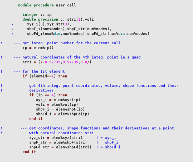
Element Coordinates and Interpolation Data at Specific Locations
The following element properties (Table 2.9: Element Coordinates and Interpolation Data) require you to specify the location where the property is calculated:
elem%
item(loc)where:
itemname of the element property.
loclocation within the element:
none = nodes. 0 = centroid. ip = integration point number. (s,t,r) = natural coordinates of a point within the element.
Table 2.9: Element Coordinates and Interpolation Data
item | Description | Location | Result Type |
|---|---|---|---|
| xyz[a] | X, Y, Z coordinates | nodes none | dp ar(3,num%nodes) |
| centroid 0 - int sc |
dp ar(3) | ||
| integration point number ip - int sc |
dp ar(3) | ||
| arbitrary point with natural coordinates (s,t,r) - dp ar(3) |
dp ar(3) | ||
| shpF | shape functions |
centroid 0 - int sc integration point number ip - int sc arbitrary point with natural coordinates (s,t,r) - dp ar(3) | dp ar (num%nodes) |
| shpFd[a] | shape function derivatives | dp ar (num%dim,num%nodes) | |
| B | strain-displacement matrix | integration point number ip - int sc | dp ar (num%compn,num%u_rows) |
| rot[b] | field or flux rotation matrix | dp ar (num%comp,num%comp) | |
| trot[b] | strain or stress rotation matrix | dp ar (num%compn,num%compn) | |
| vol[a] | volume | integration point number ip - int sc | dp sc |
Perform Operations on a Set of Scalar Nodal Values
You can also perform the following operations on a set of scalar nodal values.
Midside node interpolation
call elem%midnod(
nodes,var)where:
nodeslist of element nodes with missing midside nodes (in).
vararray of nodal variables to be interpolated (in/out).
This subroutine modifies the array of nodal variables (
var) by filling up the missing midside node entries with interpolated values.Table 2.10: Element Midside Node Interpolation
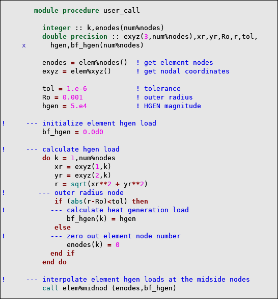
Name Description Input Type Input / Output Type midnod midside node interpolation int ar(num%nodes) dp ar(num%nodes) The following example mimics a heat generation body load defined on the outer radius of a circular 2D model.
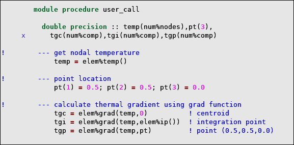
Gradient calculation
elem%grad(
var,loc)where:
vararray of nodal variables.
loclocation within the element:
0 = centroid. ip = integration point number. (s,t,r) = natural coordinates of a point within the element.
The resulting gradient vector array is in the global coordinate system. It can be rotated to the element coordinate system using the rotation utility procedures discussed in Rotate Material Matrices and Element Results Vector.
Table 2.11: Element Gradient Operation
Name Description Input Type Location loc- Input TypeResult Type grad gradient dp ar(num%nodes) centroid 0 - int sc
dp ar(num%nodes) integration point number ip - int sc
arbitrary point with natural coordinates (s,t,r) - dp ar(3)
Access Nodal and Element Results
You can access nodal and element results using the elem type-bound procedures (see Table 2.13: Element Results).
elem%
item(loc)where:
itemname of the element result
loclocation within the element:
none = nodes. 0 = centroid. ip = integration point number. (s,t,r) = natural coordinates of a point.
Table 2.12: Nodal Results
itemDescription | Location | Result Type |
|---|---|---|
| nodes none | dp ar(num%dim,num%nodes) |
| centroid 0 - int sc | dp ar(num,%dim) | |
| integration point number ip - int sc | dp ar(num,%dim) | |
| arbitrary point with natural coordinates (s,t,r) - dp ar(3) | dp ar(num,%dim) | |
| nodes none | dp ar(num%nodes) |
| centroid 0 - int sc | dp sc | |
| integration point number ip - int sc | dp sc | |
| arbitrary point with natural coordinates (s,t,r) - dp ar(3) | dp sc | |
Table 2.13: Element Results
itemDescription | Location | Result Type |
|---|---|---|
| nodes none | dp ar(num%compn,num%nodes) |
| centroid 0 - int sc | dp ar(num%compn) | |
| integration point number ip - int sc | dp ar(num%compn) | |
| arbitrary point with natural coordinates (s,t,r) - dp ar(3) | dp ar(num%compn) | |
| nodes none |
dp ar(num%comp,num%nodes) |
| centroid 0 - int sc | dp ar(num%comp) | |
| integration point number ip - int sc | dp ar(num%comp) | |
| arbitrary point with natural coordinates (s,t,r) - dp ar(3) | dp ar(num%comp) | |
Nodal DOF results are available at the start of the element calculations (Figure 2.6: Element Results Calculation Workflow) before any physics prep and integration loop. Derived results, such as strains and stresses, fields and fluxes are calculated in the sequence shown in Figure 2.6: Element Results Calculation Workflow.
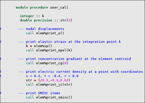
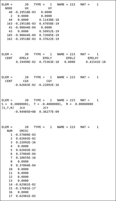
Print Formatted Element Results
You can print element results in a formatted way using the elem type-bound print procedures (see Table 2.14: Print Element Results).
call elem%print_
item(loc)where:
itemname of the element result.
loclocation within the element:
none = nodes. 0 = centroid. ip = integration point number. (s,t,r) = natural coordinates of a point. Note: elem%print_ routines are not supported for simulations using distributed-memoy parallel (DMP) processing.
Table 2.14: Print Element Results
item | Description | Location |
|---|---|---|
| u | displacement |
nodes none centroid 0 - int sc integration point number ip - int sc (s,t,r) arbitrary point with natural coordinates (s,t,r) - dp ar(3) |
|
temp volt conc |
temperature electric potential concentration | |
|
eptt epel epth epdi eppl s |
total strain elastic strain thermal strain diffusion strain plastic strain stress | |
|
tg tf ef jc cg df |
thermal gradient thermal flux electric field electric current concentration gradient diffusion flux | |
| smisc | summable miscellaneous | - |
| nmisc | non-summable miscellaneous |
Access Element Matrices and Load Vectors
You can use the following elem procedures (see Table 2.15: Element Matrices and Vectors) to access element matrices (stiffness, mass, damping, and stress-stiffness) and load vectors (applied and restoring):
call elem%
item(subscript[,subscript2])where:
itemname of the element matrix or load vector.
subscriptelements of the finite element matrix or load vector:
none = whole matrix or load vector. 0 = centroid. integer scalar(s) = single element of the matrix or load vector. vector of integers = submatrix or subvector of the matrix or load vector.
Table 2.15: Element Matrices and Vectors
|
| Result | Result Type | ||||
|---|---|---|---|---|---|---|---|
K
| none | Whole matrix K[a] | dp ar(num%rows,num%rows) | ||||
| int sc i,j[b] | Matrix element K[a](i,j) | dp sc | |||||
| int ar ia,ib[b] | Submatrix K[a](ia,ib) | dp ar(size(ia),size(ib)) | |||||
F
| none | Whole force vector F[c] | dp ar(num%rows,num%rows) | ||||
| int sc i[b] | Vector element F[c](i) | dp sc | |||||
| int sc ia[b] | Subvector F[c](ia) | dp ar(size(ia)) |
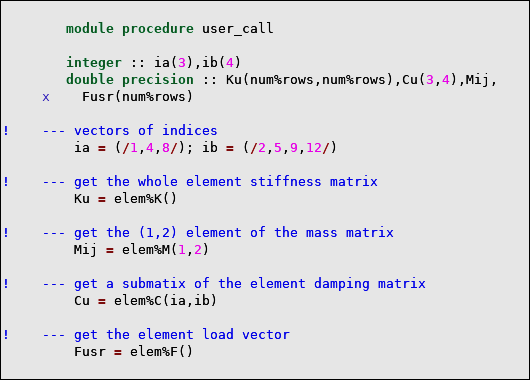
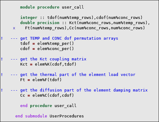
A special case of the vector subscripts are the degrees of freedom (DOFs) permutation arrays (Table 2.16: Permutation Arrays of DOFs) that indicate the positions of the DOFs within the finite element matrix or load vector.
Permutation arrays facilitate access to submatrices and subvectors corresponding to a specific physics or a coupled-field effect. They can be accessed using the following elem procedures:
elem%
item()where:
itemname of the DOFs vector subscript.
Table 2.16: Permutation Arrays of DOFs
item | Description | Result Type |
|---|---|---|
| u_per | UX, UY, and UZ DOFs | int ar(num%u_rows) |
| temp_per | TEMP DOFs | int ar(num%temp_rows) |
| volt_per | VOLT DOFs | int ar(num%volt_rows) |
| conc_per | CONC DOFs | int ar(num%conc_rows) |
Matrix and Vector Operations
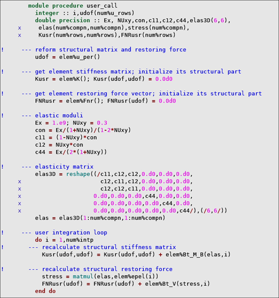
The matrix and load vector operations described in this section are used in the coupling phase of the element calculations (Figure 2.4: Element Calculation Workflow) when the physics integration loops are complete and the element matrices and load vectors are finalized. At that stage, you can write your own integration loop to customize the element matrices and load vectors.
Matrix and Load Vector Operations
The following elem procedures facilitate the calculation of element matrices and load vectors. You can call them as follows:
elem%
name(array,ip)where:
namename of the matrix-vector operation.
arrayinput:
con = constant. [M] = matrix. {V} = vector. ipintegration point number.
Table 2.17: Matrix and Vector Calculations
name | array | InputType | Result | Result Type | ||||
|---|---|---|---|---|---|---|---|---|
| N_Nt | con | dp sc |  | dp ar(num%nodes,num%nodes) | ||||
| gNt_M_gN | [M] | dp ar(num%comp,num%comp) |  | dp ar(num%nodes,num%nodes) | ||||
| gNt_V_Nt | {V} | dp ar(num%comp) |  | dp ar(num%nodes,num%nodes) | ||||
| gNt_V | {V} | dp ar(num%comp) |  | dp ar(num%nodes) | ||||
| Bt_M_B | [M] | dp ar(num%compn,num%compn) |  | dp ar(num%u_rows, num%u_rows) | ||||
| Bt_M_gN | [M] | dp ar(num%compn,num%comp) |  | dp ar(num%compn,num%comp) | ||||
| Bt_V_Nt | {V} | dp ar(num%compn) |  | dp ar(num%u_rows, num%nodes) | ||||
| Bt_V | {V} | dp ar(num%compn) |  | dp ar(num%u_rows) | ||||
where:
| ||||||||


The following example shows how the element structural stiffness matrix  and restoring force
  can be calculated using the Bt_M_B and Bt_V functions, respectively.
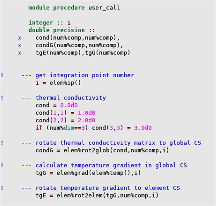
Rotate Material Matrices and Element Results Vector
When the element coordinate system is defined (ESYS) or/and geometric nonlinearities are active (NLGEOM,ON), you may need to transform material properties and element results from the element coordinate system to the global coordinate system and vice versa. With the following elem type-bound procedures, you can rotate material matrices and element results vectors to the global or to the element coordinate system. For example, material matrices and element vector results such as field and stresses must be in the global coordinate system for the element matrices and load vector calculations. On the other hand, element vector results are output in the element coordinate system.
elem%
name(array,size1,[size2],ip)where:
namename of the matrix-vector operation.
arrayinput:
[M] = matrix. {V} = vector. size1size of the square matrix [M] or vector {V}.
size2second dimension of a rectangular matrix [M].
Note: Allowed
size1andsize2:
num%comp - number of field or flux vector components
num%compn - number of strain/stress vector components
ipintegration point.
Table 2.18: Matrix and Vector Rotations
| array | size1 | size2 | Result | Input/Result Type | ||
|---|---|---|---|---|---|---|---|
| 
| num%comp |  | dp ar(size1,size1) | |||
| num%compn |  | ||||||
| num%comp | num%compn |  | dp ar(size1,size2) | ||||
| num%compn | num%comp |  | |||||

| num%comp |  | dp ar(size1) | ||||
| num%compn |  | ||||||
| 
| num%comp |  | dp ar(size1,size1) | |||
| num%compn |  | ||||||
| num%comp | num%compn |  | dp ar(size1,size2) | ||||
| num%compn | num%comp |  | |||||

| num%comp |  | dp ar(size1) | ||||
| num%compn |  | ||||||
where:
| |||||||


For example, input material properties and element calculated results (Table 2.12 Element Results) are in the element coordinate system. To rotate them to the global coordinate system when forming the element stiffness matrix or restoring force, you can use the elem%rot2glob function. On the other hand, element results such as fields and fluxes calculated from nodal degrees of freedom are in the global coordinate system. To rotate them to the element coordinate system, you can use the elem%rot2elem functions.
Process Element Matrices and Load Vectors for Missing Midside Nodes
When higher-order elements have some or all of the midside nodes dropped, element matrices and load vectors must be adjusted for missing midside nodes. The following elem subroutine modifies the element matrix or load vector by zeroing out rows (columns) corresponding to the missing midside nodes and spreading their contribution to the corner nodes rows (columns).
call elem%midnod(
array)where:
arrayinput/output:
[M] = element matrix or submatrix with nr rows and nc columns. {V} = element load vector or subvector with nr rows. Note: Allowed number of rows (nr) and columns (nc):
num%rows - total number of rows
num%u_rows – number of rows with UX, UY, and UZ DOFs
num%temp_rows – number of rows with TEMP DOFs
num%volt_rows – number of rows with VOLT DOFs
num%conc_rows – number of rows with CONC DOFs
set_ and add_ elem type-bound procedures
To define or modify materials, loads, constitutive equations, element matrices and load vectors, as well as output quantities, use the set_ and add_ elem procedures, respectively. Without the calls to these subroutines, the code in user_call has no effect on the coupled-field element behavior.
To assign a value
varto the element propertyitem, use:
call elem%set_ item_level(var)
To modify the element property
itemby adding the valuevarto it, use:
call elem%add_ item_level(var)where:
itemname of the user-programmable element quantity.
levellevel of customization:
p = data prep ip = integration point c = coupling varvariable that overwrites (set_) or is being added (add_) to the element quantity
item
User-programmable element quantities that can be defined or modified by the set_ and add_ elem procedures are listed in the following table.
Table 2.19: User-programmable Element Quantities
item | Description | level | Variable Type |
|---|---|---|---|
| tcond | thermal conductivity matrix | p | dp ar(num%comp,num%comp) |
| ip | |||
| hgen | heat generation rate | p | dp ar(num%nodes) |
| ip | dp sc | ||
| hflux | heat flux surface load | p | dp ar(num%fluxes) |
| tf | thermal flux | ip | dp ar(num%comp) |
| econd | electric conductivity matrix | p | dp ar(num%comp,num%comp) |
| ip | |||
| jc | integration point current density | ip | dp ar(num%comp) |
| diffu | diffusivity matrix | p | dp ar(num%comp,num%comp) |
| ip | |||
| csat | saturated concentration | p | dp sc |
| ip | |||
| dgen | diffusing substance generation rate | p | dp ar(num%nodes) |
| ip | dp sc | ||
| dflux | diffusion flux surface load | p | dp ar(num%fluxes) |
| df | diffusion flux | ip | dp ar(num%comp) |
| K | stiffness matrix | c | dp ar(num%rows,num%rows) |
| M | mass matrix | c | dp ar(num%rows,num%rows) |
| C | damping matrix | c | dp ar(num%rows,num%rows) |
| SS | stress-stiffness matrix | c | dp ar(num%rows,num%rows) |
| F | applied force vector | c | dp ar(num%rows) |
| Fnr | restoring force vector | c | dp ar(num%rows) |
| smisc[a] | summable miscellaneous | o | dp ar(num%smisc) |
| nmisc[a] | non-summable miscellaneous | o | dp ar(num%nmisc) |
[a] Only the set_ procedure can be used with the smisc and nmisc items.
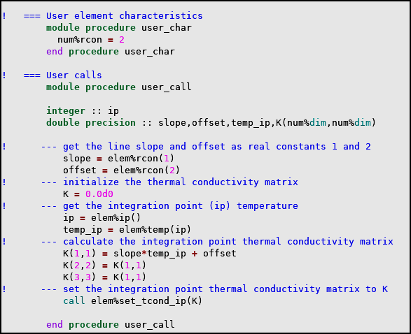
Figure 2.8: Workflows of User-programmable Quantities shows the sequence in which you can modify user-programmable element quantities listed in Table 2.19: User-programmable Element Quantities.
When modifying the user-programmable element quantities using the set_ and add_ subroutines (Table 2.19: User-programmable Element Quantities), you may need to access the nodal DOF and element calculated results. While the nodal DOF results are always available at the start of the element calculation, the element calculated results such as strains, fields, fluxes, and miscellaneous items are calculated in a sequence shown in Figure 2.6: Element Results Calculation Workflow. When calling a set_ or add_ subroutine to update a user-programmable quantity, you must ensure that any needed element results have already been calculated and are available at the time of the subroutine call.
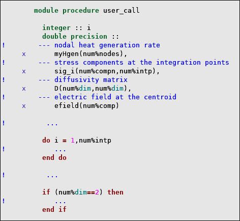
For example, when customizing thermal quantities such as thermal conductivity (tcond) or heat generation rate (hgen) in a structural-thermal-diffusion analysis, you can access structural results such as stress and elastic strain using elem%s(loc) and elem%epel(loc) functions, respectively, because the standard structural results are calculated before the thermal quantities are customized. On the other hand, standard diffusion results such as concentration gradient and diffusion flux are calculated after the customization of thermal properties, and results reported by elem%cg(loc) and elem%df(loc) during thermal calculations may not be up to date.
When a needed standard element result has not yet been calculated, you can independently derive it from the DOF solution using the element shape functions (Table 2.9: Element Coordinates and Interpolation Data) or the gradient operation (Table 2.11: Element Gradient Operation).
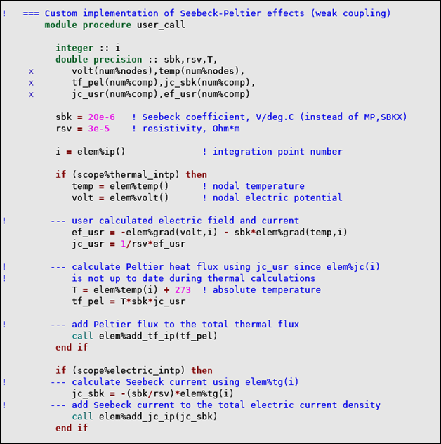
In the following example, both the thermal flux (tf) and the electric current density (jc) are customized at the integration point level to mimic the Seebeck-Peltier effects without specifying MP,SBKX that would invoke the standard coupled-field effect (Thermoelectrics in the Theory Reference). The integration point (i) thermal gradient needed for the calculation of the Seebeck electric current density (jc_usr) is already available as elem%tg(i) when elem%add_jc_ip(jc_usr) is called and does not need to be recalculated. On the other hand, the Peltier thermal flux calculation needs the total electric current density that is available only in the next (electric) stage of the element workflow (Workflow of Element Resullts Calculation (A)). To overcome this limitation, you can independently calculate the total current density (jc_usr) needed for the Peltier heat contribution to thermal flux as shown in the example below.
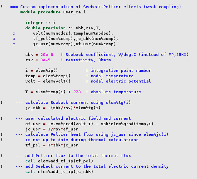
Note that the set_ and add_ procedures update the respective element variable only when the program is ready to accept it. Therefore, the sequence of these subroutines within user_call is irrelevant.
user_call procedure: solu
structure (solution settings and controls)
The structure solu
contains frequently used solution settings that you can use to control the
calculations in user_call. They can be accessed as:
solu%
itemwhere:
itemname of the solution parameter
Table 2.20: Solution Settings
Item | Description | Result Type | Result Value | ||||
|---|---|---|---|---|---|---|---|
| antype | analysis type | int sc | ANTYPE command | ||||
| nlgeom | geometric nonlinearities | int sc | 0 – off 1 – on | ||||
| nropt | Newton-Raphson option | int sc | NROPT command:
| ||||
| nrunsym | Newton-Raphson option set to UNSYM | int sc | 0 – default 1 – if NROPT,UNSYM | ||||
| xtrap | extrapolation of integration point results to element corner nodes (ERESX command) | int sc | 0 – copy 1 – extrapolate except in elements with active plasticity 2 – extrapolate | ||||
| timint | transient effects (TIMINT command) | int sc | 0 – off 1 – on | ||||
| ldstep | current load step number | int sc | |||||
| isubst | current substep number | int sc | |||||
| nsubst | maximum number of substeps | int sc | NSUBST command setting | ||||
| ieqitr | current iteration number | int sc | |||||
| neqitr | maximum number of iterations | int sc | NEQIT command setting | ||||
| output | element output pass (result calculation) | int sc | 0 – off 1 – on | ||||
| svrupd | history (state) variables update | int sc | 0 – not updated 1 – updated | ||||
| converged | converged solution | int sc | 0 – non converged 1 – converged | ||||
| time%beg | time at the beginning of the current step | dp sc | |||||
| time%end | time at the end of the current load step | dp sc | TIME command setting | ||||
| time%cur | current time value | dp sc | |||||
| time%inc | current time increment | dp sc | |||||
| time%prv | previous time value | dp sc | |||||
| time%ino | previous time increment | dp sc | |||||
| toffst | temperature offset from absolute zero to zero | dp sc | TOFFST command setting |
user_call procedure: scope
structure (scope of calculations)
The user_call procedure is called multiple times from
different parts of the element code, including every integration point of each
physics (Figure 2.4: Element Calculation Workflow). It may be inefficient to
repeat the same calculations every time the user_call
procedure is called. The components of the scope data structure allow you to narrow down the calculations to a
specific location in the element workflow.
Using the scope variables, you can limit your code to the physics, data preparation or integration loop of that physics, to a specific element quantity, or to the element output calculations:
scope%
calcscope%
calc_levelscope%
calc_level_itemwhere:
calcarea of element calculations
levellevel of customization (optional):
prep = data prep intp = integration point itemname of the user-programmable element quantity.
All variables in the scope data structure are of logical type.
Table 2.21: Parameters to Define the Scope of User Calculations
| Name | Description | Type |
| thermal | thermal calculations | log sc |
|
thermal_prep | thermal data prep | |
|
thermal_prep_tcond thermal_prep_hgen thermal_prep_hflux | input tcond, hgen, hflux calculation | |
| thermal_intp | thermal integration loop | |
|
thermal_intp_hgen thermal_intp_tcond thermal_intp_tf | integration point tcond, hgen, tf calculation | |
| electric | electric calculations | log sc |
|
electric_prep | electric data prep | |
|
electric_prep_econd | input econd calculation | |
|
electric_intp | electric integration loop | |
|
electric_intp_econd electric_intp_jc | integration point econd, jc | |
| diffusion | diffusion calculations | log sc |
|
diffusion_prep | diffusion data prep | |
|
diffusion_prep_diffu diffusion_prep_csat diffusion_prep_dgen diffusion_prep_dflux | input diffu, csat, dgen, dflux calculation | |
|
diffusion_intp | diffusion integration loop | |
|
diffusion_intp_diffu diffusion_intp_csat diffusion_intp_dgen diffusion_intp_df | integration point diffu, csat, dgen, df calculation | |
| coupling | coupled-field calculations | log sc |
|
coupling_K coupling_M coupling_C coupling_SS coupling_F coupling_Fnr | final K, M, C, and SS matrices and F and Fnr force vectors | |
| output | output calculations | log sc |
|
output_smisc output_nmisc | smisc and nmisc calculation | |
A more efficient version of the user_call Example 2.16: Customizing Thermoelectric Constitutive Equations is shown in the following example.
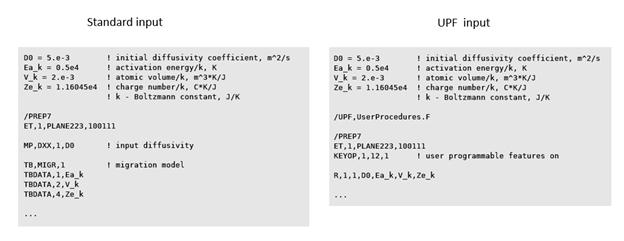
This example demonstrates the coupled-field user-programmable features (UPFs) by reproducing the standard element calculations performed when the migration model (TB,MIGR) is specified The coupled-field UPFs are activated by setting KEYOPT(12) to 1 on a coupled-field element with diffusion degrees of freedom (DOFs). The diffusion and migration parameters (D0, Ea/k, V/k, and Ze/k) are input as real constants instead of TB,MIGR that triggers the standard calculations (Figure 2.9: Standard vs. User-programmable APDL Input).
The following calculations are performed in UserProcedures.F:
the integration point diffusivity matrix D is customized using the elem%set_diffu_ip procedure
the diffusion flux constitutive equation is customized to include stress-migration flux (df_s) and electro-migration flux (df_e), and added to the total diffusion flux using the elem%add_df_ip procedure
The summable miscellaneous items corresponding to the pure diffusion flux (DFCX, DFCY, DFCZ,DFCSUM ), stress-migration flux (DFSX, DFSY, DFSZ, DFSSUM), and electro-migration flux (DFEX, DFEY, DFEZ,DFESUM), respectively, are calculated at the element centroid and output using the elem%set_smisc_o procedure
*deck,UserProcedures       USERDISTRIB       parallel
      submodule (UserInterface) UserMigr

#include "impcom.inc"

      contains

        module procedure user_char
           num%rcon = 5           ! number of real constants
           non%lin = 1            ! nonlinear analyses
        end procedure user_char

        module procedure user_call
           integer :: i
           double precision :: D0,Ea_k,V_k,Z_k,C,T,Dt,
     x       D(num%dim,num%dim),
     x       stress(num%compn,num%nodes),sigH(num%nodes),
     x       df_c(num%comp),df_s(num%comp),df_e(num%comp),
     x       df_s_m,df_e_m,df_c_m,smisc(num%smisc)

!      --- get migration parameters as real constants
           D0 = elem%rcon(2)      ! initial diffusivity coefficient
           Ea_k = elem%rcon(3)    ! activation energy/Boltzmann constant
           V_k = elem%rcon(4)     ! atomic volume/Boltzmann constant
           Z_k = elem%rcon(5)     ! charge number/Boltzmann constant

!      --- nodal stress
           stress = elem%s()
!      --- hydrostatic stress
           sigH = (stress(1,:) + stress(2,:) + stress(3,:))/3.

!      --- integration point:
           if (scope%diffusion_intp) then
              i = elem%ip()          ! number
              C = elem%conc(i)       ! concentration
              T = elem%temp(i) + solu%toffst   ! temperature
              Dt = D0*exp(-Ea_k/T)   ! diffusivity
              D = 0.0d0              ! diffusivity matrix
              D(1,1) = Dt; D(2,2) = Dt; D(3,3) = Dt

!         --- set integration point diffusivity
              call elem%set_diffu_ip(D)

!         --- hydrostatic stress gradient driven migration
              df_s = (V_k*C/T)*matmul(D,elem%grad(sigH,i))

!         --- electric field driven migration
              df_e = (Z_k*C/T)*matmul(D,elem%ef(i))

!         --- add df_s to the total diffusion flux
              call elem%add_df_ip(df_s)

!         --- add df_e to the total diffusion flux
              call elem%add_df_ip(df_e)
           end if

!      --- centroidal calculations
           if (scope%output) then
              C = elem%conc(0)       ! concentration
              T = elem%temp(0) + solu%toffst   ! temperature
              Dt = D0*exp(-Ea_k/T)   ! diffusivity

!         --- fluxes
              df_c = -Dt*elem%grad(elem%conc(),0)
              df_s = Dt*V_k*C*elem%grad(sigH,0)/T
              df_e = Dt*Z_k*C*elem%ef(0)/T

!         --- magnitudes
              df_c_m = sqrt(dot_product(df_c,df_c))
              df_s_m = sqrt(dot_product(df_s,df_s))
              df_e_m = sqrt(dot_product(df_e,df_e))

!         --- save magnitudes of diffusion fluxes as smiscs
              smisc = elem%smisc()    ! copy standard smisc
!         --- store diffusion flux
              smisc(2) = df_c(1)
              smisc(3) = df_c(2)
              if (num%comp==3) smisc(4) = df_c(3)
              smisc(5) = df_c_m
!         --- store stress migration flux
              smisc(6) = df_s(1)
              smisc(7) = df_s(2)
              if (num%comp==3) smisc(8) = df_s(3)
              smisc(9) = df_s_m
!         --- store electric migration flux
              smisc(14) = df_e(1)
              smisc(15) = df_e(2)
              if (num%comp==3) smisc(16) = df_e(3)
              smisc(17) = df_e_m

              call elem%set_smisc_o(smisc)
              if (solu%isubst==10) call elem%print_smisc()
           end if

        end procedure user_call

end submodule UserMigrThis example demonstrates the coupled-field user-programmable features (UPFs) by reproducing the effect of plastic heating normally invoked by specifying the Taylor-Quinney coefficient on the MP,QRATE command.
The following calculations are performed in UserProcedures.F:
The plastic work is calculated at each integration point using stress and plastic strain from the previous and current converged substeps.
The integration point plastic heat generation rate is:
calculated from the plastic work and premultiplied by the Taylor-Quinney coefficient (input as real constant 2)
accumulated in the elem%uwrk array for the element average plastic heat rate calculation
added to the integration point heat generation rate using the call to the elem%add_hgen_ip procedure
Current stress and plastic strain are stored on the .esav file using the elem%usvr array
User-calculated plastic heat rate is stored as NMISC,6 output item
*deck,UserProcedures       USERDISTRIB       parallel
      submodule (UserInterface) PlasticHeat

#include "impcom.inc"

      contains

!   === User element characteristics
        module procedure user_char
!     --- number of real constants
          num%rcon = 2
!     --- number of saved variables =
!         (max stress comp + max strain comp + hgen)*max integ. points
          num%usvr = (6*2 + 1)*14
!     --- number of work variables
          num%uwrk = 1
        end procedure user_char

!   === User calculations
        module procedure user_call

          integer :: i,ncomp,ns,ne,nh
          double precision :: qrate,plwrk,hgeni,
     x      s0(num%compn),s1(num%compn),
     x      ep0(num%compn),ep1(num%compn),
     x      misc(num%nmisc)

!     --- number of stress/strain components
          ncomp = num%compn

!     --- get Taylor-Quinney coefficient input as real const 2
          qrate = elem%rcon(2)

!     --- initialize work variable
          if (elem%scope%thermal_prep_hgen) then
            elem%uwrk(1) = 0.0d0
          end if

!     === Thermal integration loop
          if (elem%scope%thermal_intp_hgen) then

!       --- initialize integ. point heat generation rate
            hgeni = 0.0d0

!       --- get the integ. point number
            i = elem%ip()

!       === For a converged solution:
            if (solu%output) then       ! or solu%svrupd
!         --- get integ. point stresses and plastic strains
              s1 = elem%s(i)
              ep1 = elem%eppl(i)

!         --- pointer to saved variables
              ns = (i-1)*(2*ncomp+1) + 1
              ne = ns + ncomp
              nh = ne + ncomp

!         --- get saved stress and plastic strain
              s0 = elem%usvr(ns:ns+ncomp)
              ep0 = elem%usvr(ne:ne+ncomp)

!         --- calculate plastic work and rate
              plwrk = 0.5d0*dot_product(s1+s0,ep1-ep0)
              hgeni = qrate*plwrk/solu%time%inc

!         --- accumulate integration point hgen in the work array
              elem%uwrk(1) = elem%uwrk(1) + hgeni

!         --- save integ. point stresses, plastic strains, and hgen
              elem%usvr(ns:ns+ncomp) = s1
              elem%usvr(ne:ne+ncomp) = ep1
              elem%usvr(nh) = hgeni
            end if

!       === For each iteration:
!       --- get saved integ. point plastic heat rate
            nh = i*(2*ncomp + 1)
            hgeni = elem%usvr(nh)

!       --- add plastic heat rate to hgen
            call elem%add_hgen_ip(hgeni)
          end if

!     === Element output:
          if (scope%output) then
!       --- copy standard miscellaneous items
            misc = elem%nmisc()
!       --- output average element plastic heat rate as NMISC,6
            misc(6) = elem%uwrk(1)/num%intp
!       --- write user nmisc items
            call elem%set_nmisc_o(misc)
          end if

        end procedure user_call

      end submodule PlasticHeat
The above UserProcedures.F can be used with any coupled-field
analysis with structural and thermal degrees of freedom that supports the
UPFs.
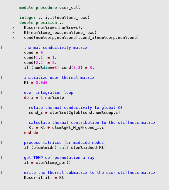
This example demonstrates the customization of the diffusing substance generation rate (dgen) in a coupled-field element with concentration degrees of freedom. The following calculations are performed in UserProcedures.F:
User-defined dgen load is calculated as a function of concentration at each element node and assigned using the elem%set_dgen_p procedure.
To enhance the solution convergence, a tangent contribution from dgen to the element stiffness matrix is calculated from the derivative of dgen with respect to the concentration
 and the array of shape functions
  as
as  using the function elem%N_Nt and added to the element stiffness matrix using the call to the elem%add_K_c procedure.
*deck,UserProcedures       USERDISTRIB       parallel
      submodule (UserInterface) UserDgen

#include "impcom.inc"
        double precision, parameter :: a = 0.05
      contains

!   === User element characteristics
        module procedure user_char

        end procedure user_char

!   === User calls
        module procedure user_call

          integer :: i,cdof(num%conc_rows)
          double precision :: udgen(num%nodes),ddgen_dC,
     x      Kusr(num%rows,num%rows)

!     --- User nodal dgen = a*conc
          if (elem%scope%diffusion_prep_dgen) then
            udgen = a*elem%conc()
            call elem%set_dgen_p(udgen)
          end if


!     --- form tangent contribution of dgen to the stiffness matrix
          if (elem%scope%coupling) then

!       --- CONC dof positions in the element matrix
            cdof = elem%conc_per()

!       --- initialize and calculate user stiffness Kusr as
!           calculate Kusr = integral(N*ddgen_dC*transpose(N)*d(vol))
!           where: ddgen_dC - derivative of dgen with respect to conc,
!                  N - shape functions,
!                  d(vol) - integration point volume
            Kusr = 0.0d0
!       --- integration loop
            do i = 1,num%intp
              ddgen_dC = a
              Kusr(cdof,cdof) = Kusr(cdof,cdof) - elem%N_Nt(ddgen_dC,i)
            end do

!       --- process Kusr for dropped midsize nodes
            if (elem%midn) call elem%midnod(Kusr)

!       --- add dgen tangent to the element stiffness matrix
            call elem%add_K_c(Kusr)
          end if

        end procedure user_call

      end submodule UserDgen
This example demonstrates the use of the displacement permutation array and element matrices by mimicking the calculation of the alpha and beta damping matrix.
The following calculations are performed in UserProcedures.F:
The user-defined damping matrix C is calculated from the element mass M and stiffness K matrices as C = alpd*M + betd*K and added to the element damping matrix using the call to the elem%add_C_c procedure.
The user-defined damping matrix C is then added to the element damping matrix through the call to the elem%add_C_c procedure.
*deck,UserProcedures       USERDISTRIB       parallel
      submodule (UserInterface) UserDamping

#include "impcom.inc"

      contains

!   === User element characteristics
        module procedure user_char
!     --- set the number of real constants
          num%rcon = 3
        end procedure user_char

!   --- Calculate user damping
        module procedure user_call

          integer :: i,udof(num%u_rows)
          double precision :: alpd, betd,Cusr(num%rows,num%rows),
     x      Kuu(num%u_rows,num%u_rows),Muu(num%u_rows,num%u_rows)

          if (elem%scope%coupling) then
!       --- get displacement dof ordering
            udof = elem%u_per()

!       --- extract structural part from the element stiffness matrix
            Kuu = elem%K(udof,udof)

!       --- extract structural part of the element mass matrix
            Muu = elem%M(udof,udof)

!       --- get alpha and beta damping factors as real constants 2 and 3
            alpd = elem%rcon(2)
            betd = elem%rcon(3)

!       --- initialize user damping matrix
            Cusr = 0.0d0
!       --- add alpha and beta structural damping to the user damping matrix
            Cusr(udof,udof) = alpd*Muu + betd*Kuu

!       --- add user damping to the element damping matrix
            call elem%add_C_c(Cusr)
          end if

        end procedure user_call

      end submodule UserDamping
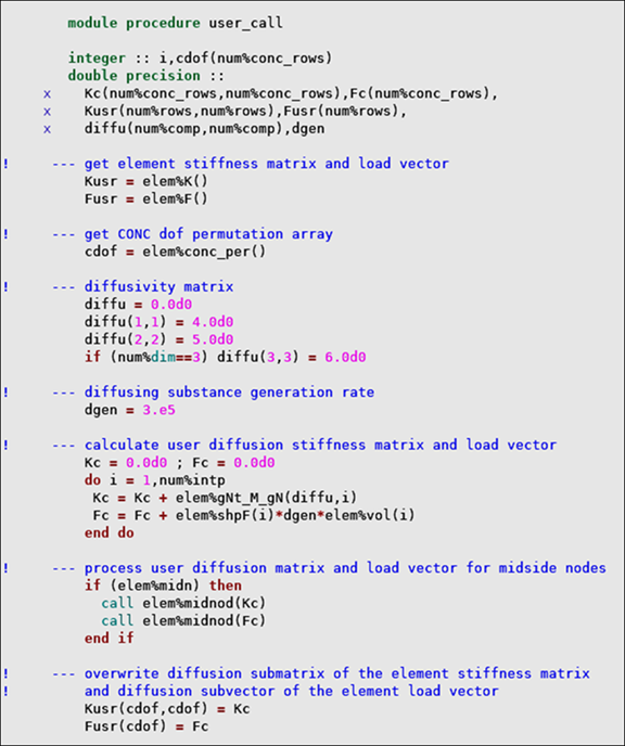
This example demonstrates the customization of diffusivity in a coupled-field analysis with concentration degrees of freedom and the calculation of the respective tangent matrix. The following calculations are performed in UserProcedures.F:
User-defined diffusivity
 is calculated at each integration point as
 , where
  is concentration.
  and
and  are input as real constants 2 and 3, respectively, and
assigned using the elem%set_diffu_ip
procedure.
are input as real constants 2 and 3, respectively, and
assigned using the elem%set_diffu_ip
procedure.The above operation is sufficient for the element to use custom diffusivity. However, to have robust solution convergence, the tangent contribution from the diffusivity is calculated from the derivative of D with respect to the concentration
 as
as  . This calculation is performed in the user integration
loop using the function elem%gNt_V_Nt
and added to the element stiffness matrix by calling elem%add_K_c. Note that for higher-order
elements, the tangent matrix is processed for the midside nodes (call
elem%midnod) before being added to
the element stiffness matrix.
. This calculation is performed in the user integration
loop using the function elem%gNt_V_Nt
and added to the element stiffness matrix by calling elem%add_K_c. Note that for higher-order
elements, the tangent matrix is processed for the midside nodes (call
elem%midnod) before being added to
the element stiffness matrix.
*deck,UserProcedures       USERDISTRIB       parallel
      submodule (UserInterface) UserDiffu

#include "impcom.inc"
      contains

!   === User element characteristics
        module procedure user_char
          num%rcon = 3    ! number of real constants
          non%lin = 1     ! nonlinear analysis
          non%sym = 1     ! unsymmetric matrix
        end procedure user_char

!   === User calls
        module procedure user_call

          integer :: i,cdof(num%conc_rows)
          double precision :: d0,a,udiffu(num%dim,num%dim),
     x       ddiffu_dC,Ktan(num%rows,num%rows),vtan(num%comp)

!     --- read real constants
          d0 = elem%rcon(2)
          a = elem%rcon(3)

!     --- user integration point diffusivity as a function of CONC
          if (elem%scope%diffusion_intp_diffu) then
!       --- integration point number
            i = elem%ip()

!       --- initialize diffisivity matrix
            udiffu = 0.0d0

!       --- calculate isotropic diffusivity diffu = d0 + a*CONC
            udiffu(1,1) = d0 + a*elem%conc(i)
            udiffu(2,2) = udiffu(1,1)
            if (num%dim==3) udiffu(3,3) = udiffu(2,2)

!       --- define user diffusivity
            call elem%set_diffu_ip(udiffu)
          end if

!     --- form diffusivity tangent contribution Ktan to the stiffness matrix
          if (elem%scope%coupling) then

!       --- CONC dof positions in the element matrix
            cdof = elem%conc_per()

!       --- initialize tangent matrix
            Ktan = 0.0d0

!       --- user integration loop
            do i = 1,num%intp
!         --- derivative of diffusivity with respect to CONC
              ddiffu_dC = a

!         --- multiply by grad(C)
              vtan = ddiffu_dC*elem%cg(i)

!         --- rotate vtan to global
              vtan = elem%rot2glob(vtan,num%comp,i)

!         --- form Ktan
              Ktan(cdof,cdof) = Ktan(cdof,cdof) + elem%gNt_V_Nt(vtan,i)
            end do

!       --- process Ktan for dropped midsize nodes
            if (elem%midn) call elem%midnod(Ktan)

!       --- add diffusivity tangent to the element stiffness matrix
            call elem%add_K_c(Ktan)
          end if

        end procedure user_call

      end submodule UserDiffu