


SHELL229
4-Node Coupled-field Shell
SHELL229 Element Description
SHELL229 is a 3D layered shell element having in-plane thermal and electrical capabilities (membrane behavior) and it supports the thermal-electric physics combination. The element has four nodes with no limitation on the number of material layers (defined by the SECDATA command). It has two degrees of freedom at each node, temperature and voltage. SHELL229 generates temperatures that can be passed to structural shell elements in order to model thermal strain. See SHELL229 in the Mechanical APDL Theory Reference for more details about this element. For verification examples, see VM215.
If the model containing the thermal-electric shell element is to be analyzed structurally, use an equivalent structural shell element instead (SHELL181 or SHELL281).
Figure 229.1: SHELL229 Geometry
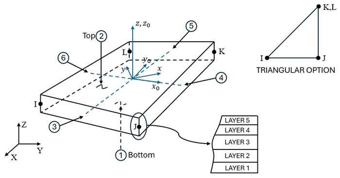
xo = element x-axis if ESYS is not supplied.
x = element x-axis if ESYS is supplied.
SHELL229 Input Data
The geometry, node locations, and coordinates systems for this element are shown in Figure 229.1: SHELL229 Geometry. The element is defined by four nodes, one thickness per layer, a material angle for each layer, and the material properties.
The cross-sectional properties are input using the SECTYPE,,SHELL and SECDATA commands. These properties are the thickness, material number, and orientation of each layer. The number of integration points through the thickness is always 1, irrespective of the number entered in the SECDATA command. Real constants are not used for this element.
The default orientation for this element has the S1 (shell surface coordinate) axis aligned with the element's first parametric direction at its center.
The default first surface direction S1 can be reoriented in the element reference plane (as
shown in Figure 229.1: SHELL229 Geometry) using the ESYS command. You
can further rotate S1 by angle THETA (in degrees) for each layer via
the SECDATA command to create layer-wise coordinate systems. See Coordinate Systems for details.
KEYOPT(1) determines the element degree-of-freedom (DOF) set and the corresponding force labels and reaction solution. KEYOPT(1) is set equal to the sum of the field keys shown in Table 229.1: SHELL229 Field Keys. Only KEYOPT(1) = 110 is supported and it activates a thermal-electric analysis with TEMP and VOLT as DOF labels and heat flow and electric current as reaction solutions.
Table 229.1: SHELL229 Field Keys
| Field | Field Key | DOF Label | Force Label | Reaction Solution |
|---|---|---|---|---|
| Thermal | 10 | TEMP | HEAT | Heat Flow |
| Electric Conduction | 100 | VOLT | AMPS | Electric Current |
The coupled-field analysis KEYOPT(1) settings, DOF labels, force labels, reaction solutions, and analysis types are shown in the following table.
Table 229.2: SHELL229 Coupled-Field Analysis
| Coupled-Field Analysis | KEYOPT(1) | DOF Label | Force Label | Reaction Solution | Analysis Type |
|---|---|---|---|---|---|
| Thermal-Electric | 110 | TEMP, VOLT | HEAT, AMPS | Heat Flow, Electric Current | Static, Full Transient |
As shown in the following table, material property requirements consist of those required for the individual fields (thermal and electric conduction) and those required for field coupling.
Table 229.3: SHELL229 Material Properties and Material Models
| Coupled-Field Analysis | KEYOPT(1) | Material Properties and Material Models | |
|---|---|---|---|
| Thermal-Electric | 110 | Thermal | KXX, KYY, KZZ, DENS, C, ENTH, HF |
| Electric | RSVX, RSVY, RSVZ | ||
| Coupling | –- | ||
The density, thermal conductivity, specific heat, and electrical resistivity can all be defined either with the MP command or the TB command.
The electrical resistivity can be defined as a function of primary variables by using tabular input on the MP command. For more information, see Defining Linear Material Properties Using Tabular Input in the Material Reference. Alternatively, TB,ELEC can be used to define electrical resistivity with TBOPT = RSV or electrical conductivity with TBOPT = COND. For more information, see Anisotropic Electrical Conductivity.
Nodal loads are defined with the D and F commands.
Element loads are described in Element Loading. Loads may be input on the element faces indicated by the circled numbers in Figure 229.1: SHELL229 Geometry using the SFE command. Body loads may be input at the element's material layers using the BFE commands.
SHELL229 surface and body loads are given in the following table. Most surface and body loads can be defined as a function of primary variables by using tabular input. For more information, see Applying Loads Using Tabular Input in the Basic Analysis Guide and the individual surface or body load command description in the Command Reference.
Table 229.4: SHELL229 Surface and Body Loads
| Coupled-Field Analysis | KEYOPT(1) | Load Type | Load | Command Label |
|---|---|---|---|---|
| Thermal-Electric | 110 | Surface | Convection Heat Flux Radiation | CONV HFLUX RDSF |
| Body |
Heat generation on material layers HG(1), HG(2), . . . , HG(number of layers) | HGEN |
The surface loads are input on a per-unit-area basis at all six faces including the shell edges:
Face 1 (I-J-K-L) (bottom, -z side)
Face 2 (I-J-K-L) (top, +z side)
Face 3 (J-I)
Face 4 (K-J)
Face 5 (L-K)
Face 6 (I-L)
This is in contrast to SHELL157 where surface loads on shell edges (faces 3 to 6 above) are input on a per-unit-length basis.
Radiation is not available on the shell edges. Convection and heat flux cannot be applied both on the same face. The surface loads can be defined by the SFE command only. You can also generate film coefficients and bulk temperatures using the surface effect element SURF152. SURF152 can also be used with FLUID116.
Element body loads may be input on a per layer basis. They can be defined with the BFE command only. One body load value is applied to the entire layer. If the first layer body load is input, and all others are unspecified, they default to the value specified for the first layer.
The body loads can be applied on material layers, where HG(1), HG(2), HG(3), . . . ., HG (number of material layers) can be defined with the BFE command only.
A summary of the element input is given in "SHELL229 Input Summary". A general description of element input is given in Element Input.
SHELL229 Input Summary
- Nodes
I, J, K, L
- Degrees of Freedom
Set by KEYOPT(1). See Table 229.2: SHELL229 Coupled-Field Analysis. - Material Properties
- Surface Loads
- Body Loads
- KEYOPT(1)
Element degrees of freedom. See Table 229.2: SHELL229 Coupled-Field Analysis. - KEYOPT(2)
Coupling method between the DOFs:
- 0 --
Strong (matrix) coupling. May produce an unsymmetric matrix. In a linear analysis, a coupled response is achieved after one iteration.
- 1 --
Weak (load vector) coupling. Produces a symmetric matrix and requires at least two iterations to achieve a coupled response.
- KEYOPT(7)
Evaluation of film coefficient:
- 0 --
Evaluate film coefficient (if any) at average film temperature, (TS+TB)/2.
- 1 --
Evaluate at element surface temperature, TS.
- 2 --
Evaluate at fluid bulk temperature, TB.
- 3 --
Evaluate at differential temperature, |TS-TB|.
- KEYOPT(8)
Material layer data storage:
- 0 --
Store data for bottom of bottom layer and top of top layer (default).
- 1 --
Store top and bottom data for all layers (the volume of data may be considerable).
- KEYOPT(13)
Film coefficient matrix:
- 0 --
The program determines whether to use a diagonal or consistent film coefficient matrix (default).
- 1 --
Use a diagonal film coefficient matrix.
- 2 --
Use a consistent film coefficient matrix.
- KEYOPT(15)
Specific heat matrix:
- 0 --
The program determines whether to use a diagonal or consistent specific heat matrix (default).
- 1 --
Use a diagonal specific heat matrix.
- 2 --
Use a consistent specific heat matrix.
SHELL229 Output Data
The solution output associated with the element is in two forms:
Nodal degrees of freedom included in the overall nodal solution
Additional element output shown in Table 229.5: SHELL229 Element Output Definitions
Output temperatures may be read by structural shell elements SHELL181 and SHELL281 via the LDREAD,TEMP command.
Convection heat flux is positive out of the element; applied heat flux is positive into the element.
The element output directions are parallel to the layer coordinate system.
A general description of solution output is given in Solution Output. See the Basic Analysis Guide for ways to view results.
To see the distribution of element quantities through the thickness for this element, enter the POST1 postprocessor (/POST1), then issue /GRAPHICS,POWER and /ESHAPE,1 followed by PLESOL.
The Element Output Definitions table uses the following notation:
A colon (:) in the Name column indicates that the item can be accessed by the Component Name method (ETABLE, ESOL). The O column indicates the availability of the items in the file jobname.out. The R column indicates the availability of the items in the results file.
In either the O or R columns, “Y” indicates that the item is always available, a letter or number refers to a table footnote that describes when the item is conditionally available, and “-” indicates that the item is not available.
Table 229.5: SHELL229 Element Output Definitions
| Name | Definition | O | R |
|---|---|---|---|
| EL | Element Number | Y | Y |
| NODES | Nodes - I, J, K, L | Y | Y |
| MAT | Material number | Y | Y |
| VOLU: | Volume | Y | Y |
| XC, YC, ZC | Location where results are reported | Y | 2 |
| THERMAL-ELECTRIC ANALYSIS (KEYOPT(1) = 110) | |||
| TG:X, Y, Z, SUM | Thermal gradient components and vector magnitude | - | 1 |
| TF:X, Y, Z, SUM | Thermal flux components and vector magnitude | - | 1 |
| EF: X, Y, Z, SUM | Electric field components and vector magnitude | - | 1 |
| JC: X, Y, Z, SUM | Conduction current density components and vector magnitude | - | 1 |
| JS: X, Y, Z, SUM | Current density components (in the global Cartesian coordinate system) and vector magnitude | - | 1 |
| JHEAT | Joule heat generation per unit volume | - | 1 |
| AREA | Face area | 1 | 1 |
| HFAVG | Average film coefficient of the face | - | 1 |
| TAVG | Average face temperature | 1 | 1 |
| TBAVG | Average bulk temperature | 1 | - |
| HEAT RATE | Heat flow rate across face by convection | 1 | 1 |
| HFLXAVG | Heat flow rate per unit area across face caused by input heat flux | - | 1 |
| THICKNESS | Shell thickness | - | 1 |
Solution values are output only if calculated (based on input values).
Available only at the centroid as a *GET item.
Table 229.5: SHELL229 Element Output Definitions lists output available through the ETABLE command using the Sequence Number method. See Element Table for Variables Identified By Sequence Number in the Basic Analysis Guide and The Item and Sequence Number Table in this reference for more information. The following notation is used in Table 229.6: SHELL229 Item and Sequence Numbers:
- Name
output quantity as defined in Table 229.5: SHELL229 Element Output Definitions
- Item
predetermined Item label for ETABLE command
- FCn
sequence number for solution items for element Face n
SHELL229 Assumptions and Restrictions
Zero thickness layers are not allowed.
The tabular thickness specified by SECFUNCTION is not supported.
The Mass transport is not supported.
Nonlinear material properties are evaluated at each integration point.
This element may not be compatible with other elements with the VOLT degree of freedom. To be compatible, the elements must have the same reaction solution for the VOLT DOF. For more information, see Element Compatibility in the Low-Frequency Electromagnetic Analysis Guide.
Source current density, JS, and Joule heat, JHEAT, are available as both element and layer average values if KEYOPT(8) = 1, and only as element average values if KEYOPT(8) = 0. The layer average values can be accessed in /POST1 by issuing the LAYER command, and in /POST26 by issuing the LAYERP26 command. If either LAYER,0 or LAYERP26,0 is issued, then the element average value is printed.