


Use the solution transition method to achieve convergence in the following situations:
Rigid body motion causing lack of convergence in a static solution. This can be due to a lack of constraints or due to a loss of contact during an iteration. Both the mass matrix and algorithmic damping of the quasi-static solution help achieve convergence for this case.
Convergence difficulty due to contact chattering. The algorithmic damping of the transient solution helps to achieve convergence.
Collapse or buckling analysis. The algorithmic damping helps to achieve convergence.
Follow these recommendations when using the solution transition method:
Since the procedure relies on the mass matrix and algorithmic damping to achieve convergence when the static solution fails to converge, it is important to define density for all materials when using this method.
Important: Because SOLOPTION can be issued in a restart after the base static analysis has failed to converge, you must define the densities during the static solution. The restart framework does not permit material density to be defined in the restart analysis.
During the transient solution phase, the default backward Euler time integration (SOLOPTION,STOT, ,QUASI) is recommended since the algorithmic damping in this method helps to keep the transient solution close to the static solution.
Monitor the kinetic energy to potential energy ratio during the transient solution to make sure it is close to a static solution. You can reduce the densities and/or add damping (ALPHAD command) to lower the kinetic energy. When adding damping, also monitor the damping energy. The kinetic and damping energies are representative of the solution approximations made to achieve convergence and should be a very small percentage (<1%) of the potential energy to achieve an accurate solution.
For details about how to use adaptive mass proportional damping in complex, non-linear problems, see Using Adaptive Mass Proportional Damping
If the static solution fails to converge due to rigid body motion or due to loss of contact, it might be more efficient to use
Type= RBM or CONT on the SOLOPTION command in order to trigger the transition to a transient solution at the first occurrence of rigid body motion (RBM) or loss of contact of an entire pair (CONT). This will save on the number of iterations performed in the static solution since it will transition before the point of convergence failure.For most problems, it can be advantageous to use the SOLOPTION command during the restart. Run the static simulation as usual, but add material densities. Then issue SOLOPTION,STOT,FORC in the restart to force a transition to the quasi-static solution. This approach can help to achieve convergence.
Adaptive mass proportional damping (ALPHAD,,AUTO) is useful for solving the following types of problems:
Although slow dynamics achieved by the quasi-static method can provide stability through numerical damping and inertia terms, adaptive mass proportional damping can help to stabilize the problem. Several types of non-linear problems are hard to converge in a static implicit solution, including problems that involve local buckling or loss of contact during the iteration, and when physics dictates that constraints cannot be applied to some parts, leaving them susceptible to rigid body motion. Adaptive mass proportional damping can help these types of problems achieve convergence. It also helps them to maintain accuracy when using the SOLOPTION command to transition to quasi-static simulation or if quasi-static simulation was used to being with.
To ensure an accurate solution, the damping is adjusted at the beginning of every substep to be high enough to provide some stability but low enough that damping energy is a small fraction of the potential energy of the system. An initial damping value specified in the ALPHAD command determines the upper and lower values for the adjusted damping. This adjustment is based on the damping and potential energy ratio of the system and solution heuristics such as convergence history and deformation state.
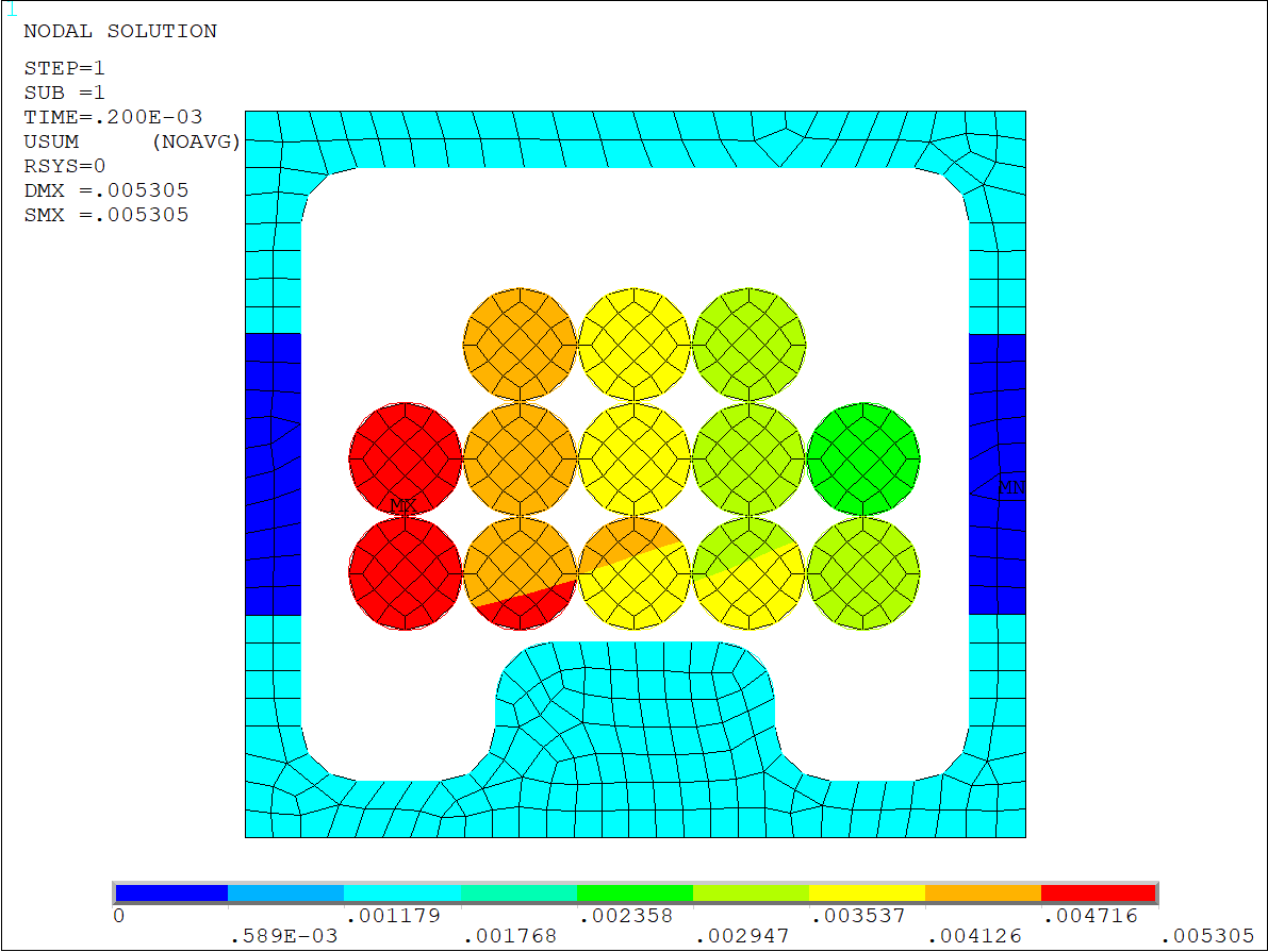
The following example shows how to use adaptive mass proportional damping in a problem where solution convergence is difficult. The sample analysis involves a two-dimensional wire crimping model, which is shown in the following figure. Initially, the wires are held together loosely. They can move freely and have rigid body motion. The static solution would therefore be hard to converge.
This problem is solved using three additional commands:
| SOLOPTION | Transtion to a quasi solution when the static solution fails to converge (default settings) |
| SOLOPTION,TTOS,TIME,0.025 | Attempt a transition back to static solution after solving the transient for 0.025 seconds, with the total load step time being 0.1 seconds |
| ALPHAD,,AUTO | Apply adaptive mass proportional damping |
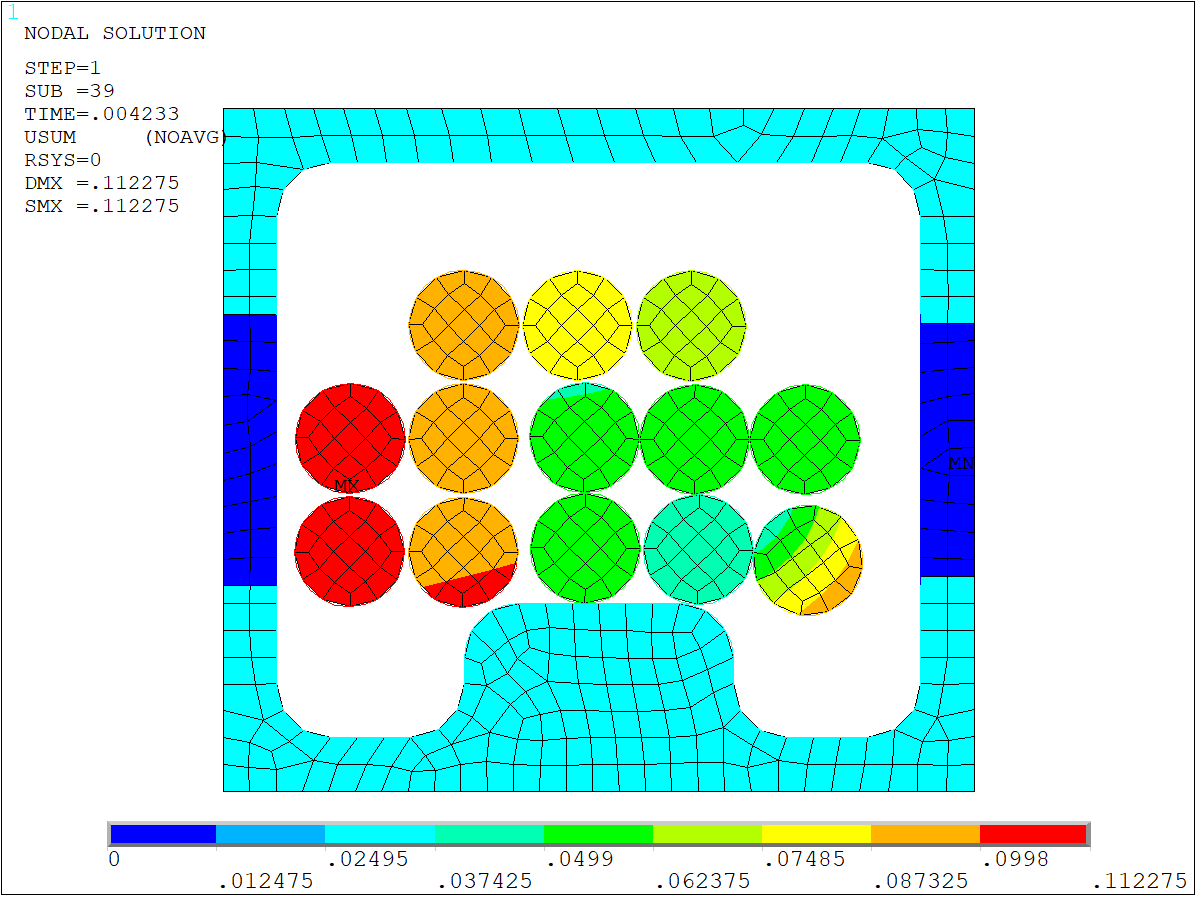
In the example problem, the static solution fails at about 4 percent of the load. The deformation history at a 4 percent load is shown in the next figure. You can see that the wires have separated from each other and will have rigid body motion, which causes the static solution to fail to converge.
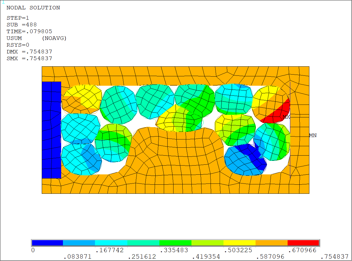
The solution automatically transitions into a quasi-static solution and solves successfully until a time of 0.08 seconds (or 80 percent of the load). The deformation state at an 80 percent load is shown in the next figure. All of the wires are in contact and are closely held together, so a static solution should converge from this time onward. In between, the quasi-static solution attempts to transition to static at every 0.025 second time interval. However, the solution is unable to converge and continues in a quasi-static phase.
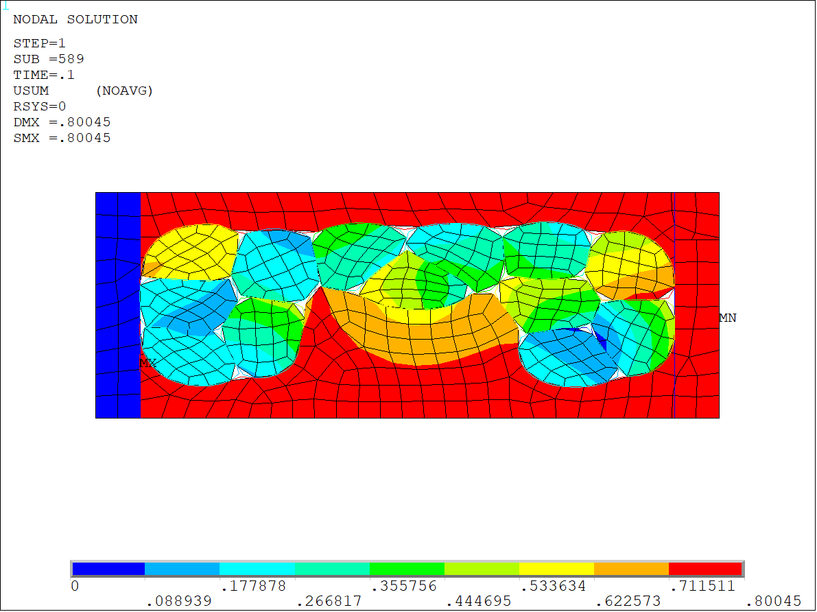
Adaptive mass proportional damping helps the solution to achieve convergence more quickly. The static solution finally converges to the deformation shown in the figure below. The number of iterations taken without any damping is approximarly twice as many as the solution with adaptive mass proportional damping, with minimal difference in the results.
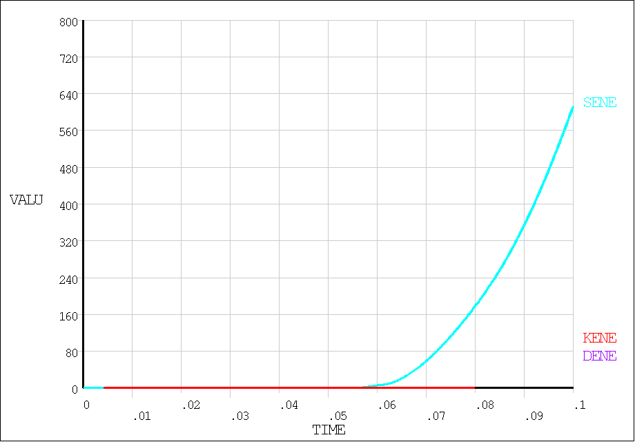
A plot of potential energy, kinetic energy, and damping energy versus time for the adaptive mass proportional damping solution is shown in the final figure. This confirms that the adaptive mass proportional damping solution stayed close to the static solution.
Figure 3.6: Potential energy, kinetic energy, and damping energy vs. time (adaptive mass proportional damping)
Keep the following in mind when using adaptive mass proportional damping in your model:
The ALPHAD command uses an initial value of 1000 as the mass multiplier to start the simulation. This value is then adjusted higher or lower to generate an accurate and robust solution. However, sometimes you may have to manually adjust the initial value of the mass multiplier. Ansys recommends using a smaller value (for example, 1) for analyses involving heavy structures.
When the SOLOPTION command is used, damping and external work are calculated during the transient phase of the solution. This information is then used to update the value of the mass multiplier. However, these quantities are not calculated from the beginning of the analysis. This means that the external work will not account for work done during the static part of the simulation.