


A 3D Look-Up Table (LUT) can be used to define field data, such as the variation of fiber directions or variable layer thicknesses. This table can be used for:
The definition of an Oriented Selection Set Reference Direction.
The definition of the draping angle (Modeling Ply).
The definition of the ply thickness (Modeling Ply).
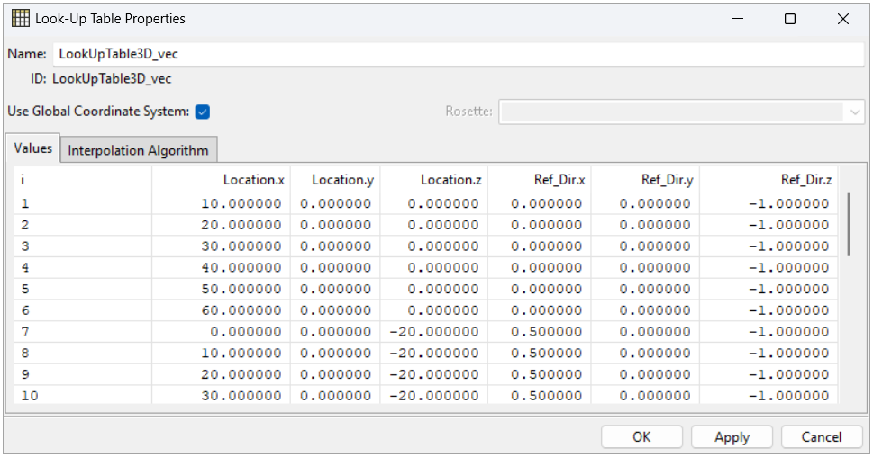
Use Global Coordinate System: If disabled, you can select a Parallel Rosette that will be used as local coordinate system for the table. In particular, the Rosette’s origin will be used as origin for the table, Rosette’s X direction will be used as the x axis and Rosette’s Y direction will be used to compute the y axis that is orthogonal to the x one. If a coordinate system is in use, it will apply to the Locations and to all the columns of the table representing a Direction. Scalar values are not affected by this option.
Rosette: Dropdown menu that enables when the “Use Global Coordinate System” is disabled and allows the selection of a Parallel Rosette as Coordinate System for the table. It is possible to leave a Rosette selected but enable Use Global Coordinate System.
Values: The values in the LUT are interpolated to the element centers. The Interpolation Algorithm tab enables you to choose between different interpolation algorithms and adjust their properties. By default, the interpolation uses the Shepard's method (a 3D inverse distance weighted interpolation) with a reasonable search radius, and the number of interpolation points is 1.
The figure below, Figure 2.45: Scalar Plot with Global Coordinate System Example, shows an example of a 3D LUT table plot with rendered support points (locations).
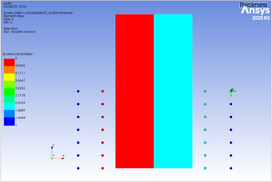
The next figure, Figure 2.46: Changed Coordinate System Translates the Support Point and Resulting Values Interpolated from the LUT, shows what happens when you select a coordinate system with a different origin and orientation. The locations for the table are transformed and the values of your model are modified accordingly. The resulting values after changing the coordinate system are particularly useful when your design changes and you must translate a LUT to another area. In that case, it is unnecessary to update the locations for accurate coordinates. All you must do is create a rosette and then use its coordinate system. Another beneficial case is when you need to apply the same LUT to various parts of your model. You can efficiently accomplish this by creating multiple copies of the same table and assigning an appropriate coordinate system to each of them, ensuring their origin and orientation are the desired ones.
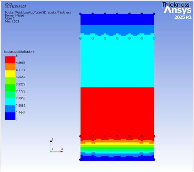
Figure 2.46: Changed Coordinate System Translates the Support Point and Resulting Values Interpolated from the LUT
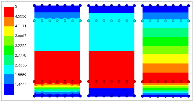
The interpolation algorithm and properties can have a significant effect on the computed values. The selection of the algorithm depends on the distribution of the supporting points and the FE mesh. The example below shows the interpolation with different algorithms for the same field. The spheres are the supporting points, and the color represents the values of the supporting points. The color of the elements represents the interpolated values. Visualize the interpolation on the mesh using the Look-Up Table Plot, which also generated these figures. For more information on interpolation, see General Interpolation Library.
Figure 2.47: Interpolated Values with Weighted Nearest Neighbor, Nearest Neighbor, and Linear Multivariate (From Left to Right)
The Look-Up Table properties are:
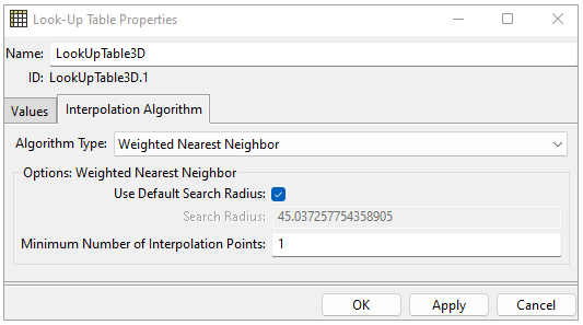
Algorithm Type: Selection of the interpolation algorithm. The supported options are Weighted Nearest Neighbor, Nearest Neighbor, and Linear Multivariate. For more details, see General Interpolation Library.
Options for Weighted Nearest Neighbor:
Use Default Search Radius: Compute the initial search radius based on the "characteristic distance" of the supported points. Validate this search radius and adjust it if needed.
Search Radius: Only the element centers within this radius are used in the interpolation.
Min. Number of Interpolation Points: If there are no element centers (or not enough if > 1) in the radius, the Search Radius increases until the pinball includes at least the minimum number of interpolation points (element centers) defined in this value.
Note: If a 3D Look-Up Table contains points without real numbers (i.e. nan or blank), these values are automatically computed on update by interpolating the valid results.