


The following sections describe the input and output files for VistaTF.exe.
- 14.2.4.1. The Auxiliary File with the Default Name: vista_tf.fil
- 14.2.4.2. Overview of Input Files
- 14.2.4.3. Overview of Output Files
- 14.2.4.4. Specification of the Control Data File (*.con)
- 14.2.4.5. Specification of the Geometry Data File (*.geo)
- 14.2.4.6. Specification of Aerodynamic Data File (*.aer)
- 14.2.4.7. Specification of Correlations Data File (*.cor)
- 14.2.4.8. Specification of the Real Gas Properties Data File (*.rgp)
- 14.2.4.9. Specification of the Output Data File (*.out)
- 14.2.4.10. Specification of the Text Data File (*.txt)
- 14.2.4.11. Specification of the CFD-Post Output File (*.csv)
- 14.2.4.12. Specification of Convergence History Data File (*.hst)
You specify the input data and output data file names in an
auxiliary data file that has the default filename vista_tf.fil. This auxiliary file in turn must contain the necessary filenames
for the input and output files in the following order and form:
Version number Version 3.0 or Version 4.0 (or newer)
control datafile name             prefix.con
geometry datafile name            prefix.geo
aerodynamic datafile name         prefix.aer
correlation datafile name         prefix.cor
results output file name          prefix.out
convergence history filename      prefix.hst
text data output file name        prefix.txt
Cfx-post output file name         prefix.csv
restart datafile name             prefix.rst
Interface output file             prefix.int
Real gas properties data file     prefix.rgp
This auxiliary file can have another name if this name is passed
to the program through a command-line argument to specify the auxiliary
filename, as described in Running Vista TF from the Command Line. If no command-line argument is specified in this way, then the
program assumes that the file has the name vista_tf.fil.
Note that the prefixes need not be identical for a given run.
In fact this is not usually the case. An example of a vista_tf.fil file is:
Version 4.0
standard_control.con
impeller_XYZa.geo
design_point.aer
radial_impeller.cor
results.out
history.hst
impeller.txt
cfx_post.csv
restart.rst
stream.int
real_gas_CO2.rgp
Note that the program also produces and uses other files in
special situations as outlined below; their names do not need to be
specified separately because they are determined by the program from
the names of other files in this list. The data files, results files,
and the file vista_tf.fil are usually in
the same directory, together with the VistaTF.bat file and the TECPLOT
layout files. If the history (.hst) file
already exists in the working directory before the program is run,
it will be overwritten. If the restart (.rst) file already exists in the working directory before the program
is run, it will be overwritten only if the solution has converged
or reached the maximum number of iterations that you have specified.
If the output (.out) file and the plot files
(.txt, and .csv)
already exist in the working directory before the program is run,
they will be overwritten. The program will not prompt you for permission to overwrite these files.
Four input data files are always needed:
Control data file (.con)
Geometrical data file (.geo)
Aerodynamic data file (.aer)
Correlations data file (.cor)
A fifth input file will be used if it is available and if you specify that it should be used:
Restart data file (.rst)
A sixth input file is needed if the calculation requires real gas properties using the Aungier-Redlich-Kwong (ARK) equation of state:
Real Gas Property data file (.rgp)
The division of the input data into separate files provides
a simple and clear way to vary or retain the annulus geometry, the
aerodynamic conditions, the blade element data, or the correlations
being used, without changing all the files in use. Typically during
the design process, you will change the .geo file to examine a new geometry, and the .aer file to examine new operating points or boundary conditions, and
you will leave the .con and .cor files untouched once you have configured their settings to meet
the requirements.
The data specified in the individual files is structured to be as logical as possible, and retains the same structure even if there is a change in the input parameters. The format of the input data is organized in such a way that most of the input files retain exactly the same format with the same parameters in the same order, without the need for a change in structure when the program changes or when the computation changes. The structure may appear more complicated than necessary, but this arises from the requirement that ultimately the program should calculate all types of turbomachinery in single stage and multistage configurations, both as ductflow and as throughflow calculations. The values of the parameters defined in the control file determine the type of data required in the other files.
An attempt has been made to include a built-in "expert system" in the program. For example, the program is able to identify whether a particular blade row is a radial compressor impeller or a radial turbine inlet guide vane (from the geometry). In general many parameters may be set to zero and the program selects the value it deems appropriate. "Expert parameters" allow you to override the selections that the program would automatically make.
The functions of the six input data files are summarized next:
Control Data File (.con)
This is a short file giving an identifier for the file (title and headers) and control information and constants defining such choices as the number of streamline calculating planes, the convergence tolerance, the relaxation factors, the number of operating points, and the number of speed lines. Various "expert" parameters are also specified in this file. Also specified in this file are the planes and stations for which output information is required, and the level of detail requested on these planes.
To make the program easier to use, you can specify many of these parameters as 0.0, 1.0, or 0, and the program will then make a sensible choice of the value for the parameter concerned, so that typically you are only concerned with two or three parameters in this file. The control parameters that determine the selection of particular numerical models are also defined in this file, for example the type of span-wise mixing or the model for blade row choking. In general, this input file does not need to be changed from run to run, except if a different number of points or speed lines are to be calculated.
Geometry Data File (.geo)
The geometry data file contains the dimensions of the annulus in terms of the axial and radial coordinates of the quasi-orthogonal calculating planes at hub and casing, and information to identify the type of calculating station (such as duct, stator, or rotor). Calculating planes can represent regions of a duct or blades (leading edges, trailing edges, and internal stations) and can be curved or linear. For linear calculating planes (which, by definition, are straight in the meridional plane), details of the geometry of each calculating plane are specified at only two points and intermediate geometric values are interpolated linearly from these, whereas curved planes require more points to be specified across the span. For curved duct calculating planes, this geometry data specifies the co-ordinate points along the curved calculating plane. In blade regions, the coordinates of the calculating plane, together with information about the blade geometry at this location, must be specified (including the number of blades, blade lean angles, and blade thickness). For each blade row, additional geometrical parameters can be specified that might be relevant for the correlations (such as the throat area, the location of the throat, the location of maximum camber, the maximum thickness, the trailing edge thickness, and the tip clearance).
In general, the geometry data file will be generated automatically
using a blade geometry definition program (such as Ansys BladeEditor, or Vista
GEO of PCA). A geometry conversion program is available to convert
data from the BladeGen meanline RTZT output
format into the .geo file format for the
throughflow program and this has been tested for radial impeller rotors
and stators, and axial stator and rotor blade rows (compressors and
turbines); see Appendix G: The RTZTtoGEO Program. Other custom
tools are available for conversion of geometrical data from specific
formats into the Vista TF .geo file format,
and others can be prepared as required.
Aerodynamic Data File (.aer)
The aerodynamic data file contains the definition of the fluid, boundary conditions, and operating data such as inlet conditions and rotational speed. It includes parameters related to aerodynamic models for the mean stream surface description, and the spanwise mixing coefficient.
Correlation Data File (.cor)
The correlation data file provides details of control parameters and empirical constants and data for the particular choice of empiricism that has been chosen. The method allows a general specification of losses, flow angle, and blockage for all calculating planes and across the span through the definition of the spanwise variation of these parameters at particular quasi-orthogonal locations and for particular blade rows. Ultimately, in many cases, if default values of zero are chosen for these parameters then the program should automatically select appropriate correlations and make its own choice of correlation parameters.
Restart Data File (.rst)
This restart file contains some key information from a previous calculation in a non-dimensional form. Note that the restart file can be for different flow conditions and for a different geometry but it must have the same number of quasi-orthogonal calculating stations and streamlines as the current calculation. If the restart data file has been generated from a calculation with similar geometry and flow conditions as the current calculation, it provides a much better initial estimate of the flow and the streamline positions than the first estimate generated internally within the program, promoting more rapid convergence. A restart with unchanged conditions and geometry will generally have a meridional velocity error of less than 2% and will converge almost immediately, except for choked flows where more iterations are needed. Convergence with the restart file is never immediate, even with unchanged geometry and flow conditions, because not all of the solution is saved to the restart file, and so some data needs to be regenerated over a few iterations of the solution. For small changes in flow conditions or geometry, the number of iterations when using the restart file is generally less than 50% of that required when starting from the program's own first estimate.
An existing restart file cannot be used if the number of streamlines or quasi-orthogonals is changed. The program recognizes if the number of streamlines or quasi-orthogonals has been changed and makes a new cold start in this case.
You do not have to be concerned with the content and format of the restart file because it is generated automatically at the end of a run of the program, and is automatically used if it is available. No further information is provided here with regards to the content of the restart file. In some situations where it is difficult to obtain convergence, the restart file can be used to store results for a converged operating point (at lower speed, for example) and then the required operating condition can be obtained by starting from the restart file with new flow conditions. In other cases where an un-converged solution has been stored in the restart file, it is possible that using the restart file can be disadvantageous as a starting point for a new simulation, and a cold-start may be better.
The restart file can also be used for reducing the number of
computations when the program is coupled to an optimizer. In this
case, an additional restart file with the name best_restart.rst is used and generated.
Real gas property data file (.rgp)
This file contains coefficients and data required to define
the gas properties of a real gas using the Aungier-Redlich-Kwong cubic
equation of state. Note that standard files have been prepared for
the most usual gases. Note this file does not have the same format
as the typical ANSYS .rgp real gas property
data files.
The program always creates the following three output files:
Results output file (
.out)Convergence history file (
.hst)Restart data file (
.rst)
In addition, when running the program for a single calculation
point at a single speed, the program can create the following output
files of tabular data for plot and display purposes, depending on
the value of the parameter i_display in the control
file:
Several comma-separated-variable output files for CFD-Post (
.csv)Several text output files in a format suitable for Tecplot (
.txt)
There is one CFD-Post output file for a calculation with no blade rows and four additional files for each blade row. There are two Tecplot output files for a calculation with no blade rows, and an additional file for each blade row.
In addition, the program can create a data file containing data in a specific format for use with other programs:
Interface output file (
.int)
and a file that can be produced as an alternative to the screen output:
Screen output file (
screen.scn)
If the program is used to calculate a performance map, the above output files are not produced, and many details of the output file are omitted and replaced by a listing of the map data.
The functions of the output data files are summarized next.
Results Output File (.out)
In single point calculations, this contains rudimentary details of the data used for the calculation and the results of the calculation at every plane and radial station for which output has been requested. In map predictions, this file contains the computed performance map. For more information, see Specification of the Output Data File (*.out).
Convergence History File (.hst)
This contains a recording of the input data, followed by details of the convergence of the main iterative procedures, and extensive details of the terms in the radial equilibrium equation for each stream tube and calculating plane. It is rare for this to be examined in any depth, but this can be useful to identify problems if the solution fails to converge. For more information, see Specification of Convergence History Data File (*.hst).
Restart Data File (.rst)
This restart file stores information from a converged calculation in a non-dimensional form. It provides a much better initial estimate of the flow and the streamline positions than the first estimate generated internally within the program. In most cases, it reduces the calculation time for a calculation with slightly modified geometry or changed aerodynamic data by more than 25%. If an existing restart file is available, it will be overwritten.
Comma Separated Variable Output Files for CFD-Post (.csv)
Depending on the value of i_display in
the control file, the following files are produced:
prefix.csvglobal_prefix.csv
together with four additional files produced for each blade row from 1 to n:
row_0n_hub_prefix.csvrow_0n_mean_prefix.csvrow_0n_tip_prefix.csvrow_0n_loading_prefix.csv
The first file (prefix.csv) contains
key results of the calculation at every calculating plane and streamline
in a form that can be used for setting up a meridional contour plot
of the results. The second contains a summary of the global performance
and reference parameters for the calculation. The additional four .csv files are produced for each blade row in the calculation.
These contain the same information as in the row data from the .txt files, but separated into hub, mean, and tip streamline
data, which is information along the blade calculating station from
leading to trailing edge on the hub, mean, and tip streamlines. The
additional file contains spanwise variation of data. This can be used
to define typical blade loading diagrams and incidence plots for each
blade row.
Even if no .csv file is required, the prefix.csv file must be specified in the vista_tf.fil file.
For more information, see Specification of the CFD-Post Output File (*.csv).
Text Data Output Files for Tecplot (.txt)
Depending on the value of I_display in
the control file, the following files are produced:
prefix.txttest_prefix.txt
together with one additional file produced for each blade row from 1 to n:
row_0n_prefix.txt
The first file (prefix.txt) contains
key results of the calculation at every calculating plane and streamline
in a form that can be used for setting up a meridional contour plot
of the results, using Tecplot software. This is an ASCII file which
is formally correct for presenting the results in graphical form with
the plot processing software Tecplot, but can be used by other plot
systems (such as Excel) with appropriate conversion or macros. A standard
layout file for Tecplot (flowfield_2d.lay) has been prepared for typical meridional plots from Vista TF calculations.
There are no macros included in this so this may need some adjustment
for a typical case (scale of axes, level of contour values, and so
on). The second text file (test_prefix.txt) contains the grid of the initial estimate of the streamlines and
quasi-orthogonals. This can be useful for debugging purposes and can
be used to plot the initial grid of an un-converged calculation to
identify any specific problems with this. The additional .txt files are produced for each blade row in the calculation
(row_0n_prefix.txt where n is the number of the blade row from the inlet). These can be used
to define typical blade loading diagrams and incidence plots for each
blade row. The Layout files for Tecplot that have been prepared in
advance assume that the .txt file has the
prefix "impeller".
Even if no .txt file is required, the prefix.txt file must be specified in the vista_tf.fil file.
For more information, see Specification of the Text Data File (*.txt).
Interface Output Files (.int)
If you request the generation of an interface file for another
analysis program then the appropriate files are also generated. The
first use of this has been established to allow a summary of the results
to be obtained as input to an optimizing software system. An option
allows the streamline locations to be printed. Even if no interface
file is required, the .int file still must
be specified in the vista_tf.fil file.
Screen Output Files (screen.scn)
In normal operation, the progress of the program can be seen
on the screen. If the command line includes a parameter -silent, the screen results will be written to a separate
file called screen.scn and not to the screen.
If this parameter is not present, the output goes to the screen. If
a name follows this parameter on the command line, the screen results
are printed to a file with this name.
The control data file includes lines of text that have no function other than to help you to identify the parameters defined here. Note that if values are set to 0.0 or 0 then standard values are used, so typically you do not have to worry about this input. If zero values are specified for some parameters then the values actually selected by the program are written to the output file. Standard forms of this file are available for editing to meet the specific requirements, whereby in most cases no modification of the file is necessary. An example of a control data file is given in Appendix C: Example of a Control Data File (*.con).
- Section 1: Character strings identifying the control data (max 72 characters/line)
The syntax is:
Character string - title(1)
Character string - title(2)
Character string - title(3)
- Section 2: Integer control parameters
The syntax is:
n_sl max_it_main max_it_mass n_points n_speeds n_reserve
Parameter
Description
n_slNumber of meridional streamlines
Notes:
Must be an odd number so that there is always a mid streamline.
Typically n = 9 or 17. If
n_sl= 0, then 9 will be used.Maximum
n_sl=max_n_sl= 29.If the mixing model is being used, (
i_mix> 0 in section 4) then there has to be a minimum of 9 streamlines.
max_it_mainMaximum number of iterations of the main streamline curvature loop in the iterative method.
Notes:
Typically specified as 500 but fewer are generally needed for simple radial compressor calculations to attain convergence.
If
max_it_main< 4 thenmax_it_main= 4, so that at least 4 iterations are always done as a minimum.If
max_it_main= 0 thenmax_it_main= 500.If the flow reaches the convergence limit before the maximum number of iterations is reached then the calculation is automatically stopped earlier.
max_it_massMaximum number of iterations for internal mass flow loop at each quasi-orthogonal calculating station.
Notes:
Typically 10 and if
max_it_mass= 0, thenmax_it_mass= 10.If
max_it_mass< 5 thenmax_it_mass= 5; experience shows that this is a sensible value.If
max_it_mass> 20 thenmax_it_mass= 20.If the mass flow convergence tolerance at a particular quasi-orthogonal is reached before the maximum number of iterations are completed then mass flow iteration is stopped early.
n_pointsNumber of points to be calculated along each speed line.
Notes:
If set to 0 or 1, then a single point is calculated.
Maximum number of points is 11.
If set to a value greater than 11, then a value of 11 will be used.
n_speedsNumber of speed lines to be calculated.
Notes:
If set to 0 or 1, then a single speed line is calculated.
Maximum number of speed lines is 11.
If set to a value greater than 11, then a value of 11 will be used.
n_reserveA further integer parameter not currently used but reserved for the possibility of defining additional data related to the map prediction (stagger schedule, bleed schedule, etc.).
Note: The last three parameters were not needed or used prior to version 4.0 of the Vista TF solver (which is the internal solver version number for Vista TF as provided with Release 15.0 of ANSYS software). If the
vista_tf.filfile being used was prepared for use with version 2 with no first line containing the version number, or was prepared for version 3 with the string "Version 3.0" in the first line, then these parameters still do not need to be specified. This allows backwards compatibility, ensuring that earlier versions will still run. These parameters will only be used if the first line of thevista_tf.filfile contains the string "Version 4.00" (or newer) in the first line. However, it is recommended that all files include these additional parameters even if they are not used.- Section 3: Integer control parameters that control input and output data
The syntax is:
i_print_plane i_print_level i_progress i_display i_restart i_interface
Note that setting all of these parameters to 0 gives a standard form of output.
Parameter
Description
i_print_planeDetermines the quasi-orthogonal calculating planes at which data is output into the results file.
= 0, as
i_print_plane= 4= 1, output at no planes
= 2, data at inlet and outlet planes only
= 3, data at leading edges and trailing edges and inlet and outlet planes only
= 4, data at all planes
Note:
The extent of the data printed at each plane is determined by
i_print_level.i_print_levelDetermines the level of output data printed into the results file at each output plane.
= 0, standard output (as
iprint_level= 3)= 1, very limited data at each plane
= 2, generous level of data at each plane
= 3, extensive data at each plane
Note:
The planes at which output is available are defined by the parameter
i_print_plane.i_progressDetermines the extent of intermediate data that is printed to the various files.
If
i_progress= 0 then no intermediate information is printed.If
i_progress= 1 then intermediate progress of the iterations are printed to the history file.If
i_progress= 2 then data is printed to the history file and to the screen.
i_displayDetermines extent of tabular data output which is prepared for displaying the results with other plot and post-processing tools:
Notes:
If
i_display= 1, then no plot files are produced.If
i_display= 0 then the output files of type .txt are produced for display of the results with Tecplot.If
i_display= 2, then a comma separated variable file with extension.csvis produced for display of the results with CFD-Post.If
i_display= 3, then bothi_display= 0 and 2 above are activated.Other output formats can be incorporated as requested.
i_restartDetermines whether the restart file should be used and whether the results will overwrite the restart file contents.
Notes:
If
i_restart= 0, the restart file (prefix.rst) will be used automatically if it is present (a warm start) and its content will be overwritten automatically at the end of a normal calculation. Note that this also overwrites the restart file even if the iterations are not converged, so that a second start with the same number of iterations starts with a better approximation. This is the normal way to use the program. The restart file includes the number of quasi-orthogonals and streamlines. Ifi_restart= 0 and this number has changed then the program makes a cold start with its own estimate of initial conditions (as ini_restart= 1).If
i_restart= 1 the restart file (prefix.rst) will not be used even if it is available and the program will set up its own initial conditions (a cold start). The content of the restart file will be overwritten as under 1 above. This is not generally recommended but can be useful in debugging difficult cases. This is equivalent to deleting the existing restart file and using option 1 above.i_restart= 2 and 3 are special options for running the program when coupled to an automatic optimizer. In these cases the use of a good restart file reduces the number of iterations needed and brings a reduction in calculating time. Unfortunately some of the geometries being examined may be poor and so it is inadvisable to overwrite the restart file with poor results. Ifi_restart= 2 then the file runs with a restart file calledbest_restart.rstand writes the results on toprefix.rst. Ifi_restart= 3 then the file runs with a restart file calledbest_restart.rstand also writes the results on to the same filebest_restart.rst. In both cases if the restart filebest_restart.rstis not present then the internal initial estimate is used (a cold start).
i_interfaceDetermines the type of output interface file that is generated.
Notes:
If
i_interface= 0 then no output interface file is generated.If
i_interface= 1 then theprefix.intfile contains a summary of the results for use in radial compressor optimization.If
i_interface= 2 then the.intfile contains the coordinates of the streamlines of the calculation.If
i_interface= 3 then the.intfile contains the coordinates of the streamlines of the calculation in a format suitable for the stream file of the blade-to-blade program MISES.
- Section 4: Integer control parameters for various models and reference parameters
The syntax is:
i_expert i_flow i_fluid i _inbc i_mass i_mix i_ree
Parameter
Description
i_expertAllows special calculations to be carried out making use of development features of the program. Normally you would set the value of this parameter to 0 or 1, but other expert features of the program may be modified with this control parameter. Each digit of the parameter has an influence on its effect.
Notes:
The last digit controls the choke calculation mode. Using a value of zero for the last digit causes the choke mass flow limitation to be eliminated which may be more robust in difficult cases. Calculations of new cases should start in this mode.
Using a value of 1 for the last digit, enables the choke mass flow limitation calculation. This requires exact data for the throat areas to be specified and should only be used if this is available. It is necessary to set this value to 1 when using iteration to pressure ratio in choked stages.
The second-last digit controls the blending function calculation for the deviation between the blade angle and the flow angle as follows:
0 - Turbines use departure angle at the leading and trailing edge ends, Compressors use swirl at the leading edge and departure angle at the trailing edge.
1 - Turbines and compressors use the departure angle for the leading and trailing edges.
2 - Turbines and compressors use departure angle at the trailing edge and relative swirl at the leading edge.
3 - Turbines and compressors use departure angle at the trailing edge and the absolute swirl at the inlet.
4 - Compressors use swirl at the leading edge and departure angle at the trailing edge; turbines use swirl at the outlet and departure angle at the leading edge.
5 - Compressors use swirl at the leading edge, departure angle at the trailing edge; turbines use swirl at the trailing edge and departure angle at the leading edge.
i_flowDetermines the input definition for the reference flow parameters (which are input in
.aerfile).Notes:
i_flow= 0 to 4 is for a calculation with a specified mass flow.i_flow= 5 to 9 is for a calculation with a specified pressure ratio. See below.i_flow= 0 thenref_mach,ref_phi, andref_d, are specified, but ifref_mach> 3 then it is interpreted asref_u, so this is equivalent toref_u,ref_phi, andref_d.i_flow= 1 thenref_n,ref_mass, andref_dare specified.Note: If there is more than one spool in the calculation with different rotational speeds, then this is taken into account as follows:
- If
i_spool= 2 andi_flow= 1 thenref_n1,ref_n2,ref_mass, andref_dare specified.- If
i_spool= 3 andi_flow= 1 thenref_n1,ref_n2,ref_n3,ref_mass, andref_dare specified.i_flow= 2 thenref_n,ref_volume, andref_dare specified.i_flow= 3 thenref_u,ref_mass, andref_dare specified.i_flow= 4 thenref_u,ref_volume, andref_dare specifiedi_flow= 5 thenref_n,ref_mass, andref_dare specified together with theref_pr(total to static pressure ratio between inlet plane and the last trailing edge on the mid-streamline). The value ofref_massis a start value for mass flow in the iteration to pressure ratio and has no effect on the final solution.i_flow= 6 thenref_n,ref_mass, andref_dare specified together withref_pr(total to static pressure ratio) together withn_p_te(the total number of trailing edges at which a guessed value of the static pressure ratio is specified, followed by the guessed pressure ratios at each trailing edge, including the last, which is also defined byref_pr.i_flow= 7 thenref_n,ref_mass, andref_dare specified together with theref_p(static pressure at the last trailing edge on the mid-streamline). The value ofref_massis a start value for mass flow in the iteration to outlet pressure and has no effect on the final solution. This option may be useful for low speed devices where pressure ratio becomes indeterminate.i_flow= 8 thenref_n,ref_mass, andref_dare specified together with theref_p(static pressure at trailing edge pane) together withn_p_te(the total number of trailing edges at which a guessed value of the static pressure is specified, followed by the guessed pressures at each trailing edge, including the last, which is also defined byref_p.i_flow= 9 thenref_n,ref_mass, andref_dare specified together with theref_cu(absolute swirl velocity at the last trailing edge on the mid-streamline). The value ofref_massis a start value for mass flow in the iteration to outlet swirl and has no effect on the final solution. This option may be useful for turbine calculations where the last blade row is a turbine rotor.The versions with specified static pressure and specified outlet swirl have not been fully tested.
Other options are available for debugging purposes but are not described here.
The geometry definition of Vista TF assumes clockwise rotation. This leads to a certain convention for the sign of the blade angles (see Appendix A: Sign Convention for Angles and Velocities in Vista TF). In some cases you may have a counterclockwise machine with blade angles of the opposite sign. To avoid the need to change all the angles specified in the
.geofile, an option is provided whereby the value ofi_flowis given a negative sign. As a more sophisticated alternative the blade speed may be defined as negative.
i_fluidDetermines the model for the equation of state of the fluid:
If
i_fluid= 0 then ideal gas with constant specific heats.If
i_fluid= 1 then liquid.If
i_fluid= 2 then a real gas calculated with the Aungier-Redlich-Kwong equations.If
i_fluid= 3 then real gas calculated with the Redlich- Kwong equations.If
i_fluid= 4 then an ideal gas calculation with variable specific heats is carried out. This is done by using the real gas equations but setting the coefficients of the Aungier-Redlich-Kwong equations to the appropriate values internally in the program to reproduce an ideal gas equation.If
i_fluid= 6 or 7 a calculation is done with a real gas with a constant real gas factor and a constant isentropic exponent.Steam properties can be approximated with the Aungier-Redlich-Kwong equations using the values of the coefficients to model steam.
i_inbcDetermines the type of inlet boundary conditions:
i_inbc= 0 then input values are total pressure, total temperature and swirl (rxcu, that is radius times circumferential component of the absolute velocity) on the input plane.i_in_bc= 1 then input values are total pressure, total temperature, and absolute flow angle.i_in_bc= 2 then input values are: total pressure, total temperature, and absolute circumferential flow velocity.
See also the section on
n_inbcin the aerodynamics file (described in Specification of Aerodynamic Data File (*.aer)) where the inlet profile across the span can be specified.i_massDetermines whether the mass flow is uniformly distributed across streamlines or not.
i_mass= 0 then the mass flow between each streamline is the same.i_mass= 1 then the fractional mass between each streamline has to be input into the last line of the control file.i_mass= 2 then the cumulative mass for each streamtube from the hub streamline is defined in the last line of the control file.
i_mixDetermines which mixing model is used:
i_mix= 0 then no mixing model.i_mix= 1 then a spanwise mixing model based on eddy diffusion across the streamlines will be used. Note that this requires a minimum of 9 streamlines (n_sl=> 9).
i_reeDetermines the form of the radial equilibrium equation that is used to determine the velocity gradient along the quasi-orthogonal.
i_ree= 0 then the equations as given in the paper of Casey and Roth (1984) are used, except that the dissipation term is set to zero and the blade force term is set to zero at a trailing edge and at a leading edge.i_ree= 1 then the solution is as fori_ree= 0 but the dissipation term is not set to zero but the equations as given in the theory documentation are used.i_ree= 2 then the dissipation term is not set to zero but the equations given in the paper of Casey and Roth (1984) are used.i_ree= 3 then the velocity gradient in the radial equilibrium equation is reduced by the factorgrad_reegiven in section 5. This is useful for debugging difficult cases and the simulation becomes similar to a mean-line calculation with no gradient of meridional velocity across the span. Ifgrad_ree= 1.0 then selectingi_ree= 3 has no effect.
- Section 5: Convergence and damping factors
The syntax is:
damp_sc damp_vl cm_start tolerance_cm tolerance_mass grad_ree
The damping factor model automatically chooses the most appropriate values of these parameters based on the type of turbomachine and the grid. You then typically need to specify the following values for this section:
0.00 0.00 0.00 0.00 0.00 1.00
In some rare cases it may still be necessary to select these values differently.
Parameter
Description
damp_scDamping factor for streamline curvature terms.
Notes:
The Wilkinson stability analysis for streamline curvature programs indicates that the streamline curvature damping term has to be reduced for long closely spaced quasi-orthogonals (high aspect ratio). For details, see the section on computational grid (Computational Grid).
If
damp_sc= 0.0 then the program determines the value of the damping factor from the theory of Wilkinson, or uses an internally determined value that differs for each type of turbomachine — whichever is smaller.Typically values of
damp_scbetween 0.05 and 0.25 are used, but lower values may be necessary for high aspect ratio quasi-orthogonals (as in end stages of steam turbines).If the specified value of
damp_scis larger than the value predicted by the Wilkinson stability theory then the program automatically reduces the damping factor to a stable value.If the program has convergence problems with an increasing error then the value is automatically reduced internally within the program during the convergence process.
Several different schemes for the damping are applied. The original scheme is obtained with a value of
damp_scbetween 1.0 and 1.25. New schemes which are more stable and robust in most cases can be obtained with the value ofdamp_scbetween 0.0 and 0.25. A value between or 2.0 and 2.25 uses the original scheme with changed constants. A value between 3.0 and 3.25 gives a very robust scheme for highly staggered blades. The first digit then defines which scheme is used (0 - new scheme, 1 - original, 2 - modified original, 3 - new scheme for highly staggered blades) and the digits after the decimal point are the damping factor (damp_sc) itself.
damp_vlDamping factor on velocity level. Note this damping factor is also used internally in the program for all parameters which are under-relaxed.
Notes:
There is no stability theory to define this, and a typical value used is 0.50, indicating that 50% of the new parameter together with 50% of its original value is used.
If
damp_vl= 0.0 then 0.50 is used.
cm_startValue of meridional velocity on the mean streamline as a fraction of
u_ref, as used in the initial conditions. This is then a sort of flow coefficient (cx/u) of the device concerned and is used as a guide to the velocity levels that can be expected.Notes:
Recommended that this should be less than the actual value when converged because this avoids choking during the early streamline curvature iterations.
If simulations from a cold-start (with no restart file) fail to converge, it may be useful to modify this parameter because it strongly influences the start velocities.
Not used if the restart initial condition is used.
If
cm_start= 0.0 then 0.25 is used for all calculations except radial turbines where 0.1 is used. The value of 0.25 is probably adequate for radial compressors only.
tolerance_cmTolerance level on change in meridional velocity during streamline curvature iterations. The value specified is the maximum percentage change in meridional velocity for convergence. Iterations stop when all streamlines and all quasi-orthogonals have a lower value than this.
Notes:
Typical value 0.01 (that is, 0.01%, which is 1 part in 10,000).
If
tolerance_cm= 0.0 then 0.01% is used.Note that if the meridional velocity is low at a certain point in the flow field, it may be necessary to use a higher value than this.
Note that the extremely low value of 0.01% does not imply that the solution is as accurate as this, but just provides confidence that convergence has really been achieved.
tolerance_massTolerance level on mass flow for internal mass flow iteration. Note that because this controls the convergence of the innermost loop, it should be a factor of 2 to 10 lower than the tolerance value for the meridional velocity (above).
Notes:
Typical value 0.001 (that is 0.001%, which is 1 part in 100000).
If
error_max= 0.0 then 0.001% is used.
grad_reeFactor to reduce the spanwise velocity gradient from the radial equilibrium equation. Normally equal to 1.0 indicating that the gradient from the radial equilibrium equation is used without change. For calculations with
i_ree= 3, ifgrad_reeis set to 0.0, the program takes a meridional velocity gradient of 0.0 (that is constant meridional velocity across the span) and a value between 1.0 and 0.0 reduces the spanwise gradient of meridional velocity determined by the radial equilibrium equation by this amount.- Section 6: Mass flow distribution between streamlines (n_sl - 1 values)
The syntax is:
f_mass_st(1), f_mass_st(2), ... f_mass_st(n_sl - 1)
Parameter
Description
f_mass_stA list of numbers expressing the relative mass flow for each stream tube.
Notes:
This line is only needed if
i_mass= 1 or 2 on line 4 of the.confile, but for consistency, it is recommended to use it in all input files.The number of values needed corresponds to the number of streamtubes, which is one less than the number of streamlines, so this line requires modification if the number of streamlines for the calculation is changed. The number of values and the values themselves need to change if the number of streamlines in the simulation is changed.
If
i_mass= 1 then this line is interpreted as the relative mass flow for each streamtube from the hub, so the values of1/(n_sl - 1)would give a uniform distribution. Each value may be specified as the relative mass flow for a streamtube compared to the sum of all values, so a value of 1.0 for each streamtube also leads to a uniform mass flow distribution.If
i_mass= 2 the cumulative values from the hub are specified, so the first value is 0.0 and the last value is 1.0.It is recommended that the distribution is selected such that the central streamline always splits the flow into two regions of equal mass flow. The reason for this is that some correlations operate on the mean streamline.
The numbers may be specified on different lines.
Note:
f_mass_stis not needed ifi_massis zero because the program will then automatically use a uniform distribution of mass flow between the streamlines. For consistency, you should use this parameter even for cases where it is not needed.
The geometry data file includes sections of text lines that help you to identify the parameters defined here. You should read the section on geometry in Appendix A: Sign Convention for Angles and Velocities in Vista TF to become familiar with sign conventions and angle definitions used in this file. An example of a geometry data file is given in Appendix D: Example of a Geometry Data File (*.geo) for a Radial Impeller.
- Section 1: Character strings identifying the geometry data (max 72 characters/line)
The syntax is:
Character string - title(1)
Character string - title(2)
Character string - title(3)
- Section 2: Number of quasi-orthogonal lines and scale factor (one line)
The syntax is:
n_qo scale
Parameter
Description
n_qon_qo= number of quasi-orthogonal lines from inlet to outlet of the domain. From version V1.31 onwards the maximum value of this parameter is unlimited.scaleThe scaling factor for all geometry data that is input.
Notes:
Usually the geometry data is input in SI units (that is, all values are expected in m and not mm) and then this value is 1.0.
If the input geometry data comes from a CAD system then it may be in mm. In this case, the value of
scalemust be 0.001. Similarly the value can be adjusted to allow the geometry data to be input in other systems of units; for example, inches.This scale factor only scales the data in the geometry input file and has no effect on other dimensions elsewhere; for example, it does not scale the reference diameter, which must be input with units of meters, in the aerodynamic file.
If you specify
scale= 0.0, unity is used.
For each quasi-orthogonal, the following data is required to define the flow channel for the meridional through-flow calculation and the meridional spacing of the quasi-orthogonals. Note that some of this data is also repeated in the section on the blade geometry. This duplication allows calculations to be made in a channel that is not the same as the hub and casing line of the actual blade definition (blade cropping or blade trimming).
- Section 3: Definition of quasi-orthogonal types and end points (n_qo lines: i = 1 to n_qo)
The syntax (of a single line) is:
i r_hub(i) r_shr(i) z_hub(i) z_shr(i) n_blade(i) n_curve(i) i_type(i) i_row(i) i_spool(i)
Parameter
Description
iNumber of a particular quasi-orthogonal line.
Notes:
The actual value is not used by the program internally because it recounts the quasi-orthogonals as they are input. You can use this number to recognize a particular line of data in the input file.
This allows you to merge two different geometry files of, say, a rotor and stator, to a single stage geometry file without the need to renumber the quasi-orthogonals. In this case, the same number may appear more than once. In a similar way, a single quasi-orthogonal may be removed without the need for renumbering the lines.
r_hub(i)Radial coordinate at hub end of quasi-orthogonal [m].
r_shr(i)Radial coordinate at casing end of quasi-orthogonal [m].
z_hub(i)Axial co-ordinate at hub end of quasi-orthogonal [m].
z_shr(i)Axial co-ordinate at casing end of quasi-orthogonal [m].
Notes on co-ordinates:
r_hubmay not be close to zero; adapt the grid if necessary to avoid small values ofr_hub.The aspect ratio of the quasi-orthogonal lines determines the stability of the solver. The lines should not be too closely spaced.
The end coordinates of the leading and trailing edges of blade rows should be included in the list of coordinates.
The end coordinates of the leading edge of a splitter vane should be included in the list of coordinates.
n_blade(i)Number of blades in blade row.
Notes:
= 0 in duct regions.
The number of blades changes at a splitter blade leading edge in a compressor or at a splitter vane trailing edge in a turbine, and changes again for multiple splitters. This is the only information that the program has about the splitters, so the location of the splitter vane leading or trailing edge needs to be a quasi-orthogonal line in the input data.
n_curve(i)Number of defining points along the
ith quasi-orthogonal line.Notes:
= 1, a special case for duct stations. This indicates that there are 2 defining points (as for
n_curve(i)= 2) but that no further information for this calculating station is provided in section 4 below, because it is already fully defined by the hub and casing points given in section 3.= 2 for a linear calculating plane in which only the end points of the quasi-orthogonal are defined. In this case, similar information can be found in section 4.
> 2 for a non-linear or curved calculating plane.
The number of defining points can vary from station to station but
n_curve(i)should typically be the same for all stations because streamline section data is usually available on a fixed number of spanwise sections.Note that the hub and casing geometry information does not necessarily have to be the same as that defined in section 4. In this case the data in section 3 will be used to crop the blade row or to make a section through the blade information in section 4.
i_type(i)Parameter to identify type of calculating station:
1 - for duct region
2 - for non-rotating blade row (stator)
3 - for rotating blade row (rotor)
Notes:
The program internally identifies which lines are leading and trailing edges from the changes of type of blade row, and which line is the leading edge of a splitter vane (by the change in blade number).
There must be at least two duct calculating stations upstream of the first blade row, and downstream of the last blade row.
A blade row must consist of at least two calculating stations (leading and trailing edge). Typically a radial impeller will have around 15 calculating stations, because this gives a 6° turn between each station and improves the calculation of the curvature terms.
There must be at least two blade calculating stations upstream and downstream of a splitter vane leading edge.
Other types of blade row may be defined at a later stage.
i_row(i)This parameter is used to identify type of blade row and stage of the quasi-orthogonal calculating station. In fact the program can usually identify the type of blade row itself from the geometry and the context, so it is not necessary to specify these values at all and, in the first instance, this parameter may be set to zero. They are included here for special cases where the program may have difficulty with the rules that are coded to identify blade row types.
= n11 - radial compressor inlet guide vane1
= n12 - radial compressor inlet guide vane2
= n13 - radial compressor impeller blade
= n14 - radial compressor diffuser vane
= n15 - radial compressor return channel vane
= n16 - radial compressor axial de-swirl vane
= n21 - axial compressor inlet guide vane1
= n22 - axial compressor inlet guide vane2
= n23 - axial compressor rotor blade
= n24 - axial compressor stator vane
= n25 - axial compressor outlet guide vane
= n31 - radial turbine inlet guide vane1
= n32 - radial turbine inlet guide vane2
= n33 - radial turbine impeller blade
= n34 - radial turbine stator vane
= n35 - radial turbine outlet guide vane
= n41 - axial turbine inlet guide vane1
= n42 - axial turbine inlet guide vane2
= n43 - axial turbine rotor blade
= n44 - axial turbine stator vane,
= n45 - axial turbine outlet guide vane
Notes:
The value of n determines which stage is being considered, such that a multistage axial compressor with an IGV would begin with values of 121 for the inlet guide vane, continue with values of 123 for the rotor, and 124 for the downstream stator, so that the next rotor would be 223, and so on. A double row of stators would be denoted as n24 and n25 for the successive blade rows.
i_spoolParameter to identify rotational speed of spool or shafts where different blade rows have different speeds.
0 single shaft with one speed (
ref_n)1 (or 0) first shaft with speed (
ref_n1)2 second spool with second speed (
ref_n2)3 third spool with third speed (
ref_n3)Note that counter-rotating blade rows can be dealt with by specifying negative speeds for the second spool. The program determines the number of different spools (
n_spool) from the number of different values ofi_spool(i)found in the geometry input file. (The maximum is set to be 3.)Notes:
The data is supplied on
n_curvelines spaced fairly evenly from hub to casing. For example, ifn_curve= 5, there may be points at 0%, 25%, 50%, 75%, and 100% of span. Ifn_curve= 2, there will be just two points, at 0% and 100% span.The blade data and quasi-orthogonal data in section 4 may extend outside of the flow channel defined by the meridional coordinates given in section 3. In a normal calculation, the data overlaps partly with that given in section 3, because the end points of the quasi-orthogonal lines are defined twice (except for duct calculating stations with
n_curve(i)= 1; see above). The flow channel defined in section 3 is generally congruent with the blade hub and shroud defined in section 4. The blade, as defined in section 4, may extend outside of the region of the flow channel because this allows a calculation to be made in a cropped or trimmed flow channel only by changing the data in section 3; section 4 does not need to be changed.The end points of the quasi-orthogonal lines, as defined by coordinates
r_hub(i),r_shr(i),z_hub(i), andz_shr(i), should lie along the quasi-orthogonal lines as defined byr_qo (j,i)andz_qo(j,i)below. In many cases, the end points will be coincident with the blade data, but if this is not the case, it is not acceptable to define end points that do not lie on the blade data point.All the angles are specified in degrees because this is more convenient in those cases where it may be necessary to define the geometry by hand, and also allows a simple consistency check, but internally the program converts them into radians. A further description of the angles is provided in Appendix A: Sign Convention for Angles and Velocities in Vista TF.
The sections above define only the hub and casing walls and provide information on the type of calculating station. The detailed orientation and position of the curved quasi-orthogonal line and the details of the blade surface geometry are provided in the next section.
- Section 4: Geometry of quasi-orthogonal lines and blade
The syntax (of a single line) is:
i j r-qo(j,i) theta_qo(j,i) z_qo(j,i) thu_qo(j,i) gamma_r_qo(j,i) gamma_z_qo(j,i)
Parameter
Description
iNumber of a particular quasi-orthogonal for data input (increasing from inlet to outlet). Note that this value is not read in as input data or used by the program but is simply used as orientation in the data file when examining the geometry input data.
jNumber of streamline for data input (increasing from hub to shroud). Note that this value is not read in as input data but is simply used as orientation in the data file when examining the geometry input data. Note that for each
q-o (i), the spanwise data is entered(j)before continuing with the nextq-o.r_qo(j,i)Radial coordinate of point
jalongq-o (i)[m].theta_qo(j,i)Circumferential coordinate of blade camber line at point (
r_qo,z_qo) [degrees].Notes:
The angular coordinate (theta) is taken as positive in the clockwise direction of rotation and negative in the other direction.
In a duct region this angle may be zero.
This angle is not used by the program but helps to visualize the blade shape and may be useful for plots of the blade shape.
In a region where there is a splitter vane this angle is the blade camber angle of the main blade and not of the splitter, or it may be defined as the mean value for both blades.
z_qo(j,i)Axial coordinate of point along quasi-orthogonal [m].
thu_qo(j,i)Circumferential thickness of blade at point (
r_qo,z_qo) [m].Notes:
In a duct region this thickness should be specified as zero.
In a region where there is a splitter vane this thickness is the mean thickness of the main blade and the splitter.
At leading and trailing edges the value supplied is not used by the program, but the calculating station is taken to be at the limit of the chord with zero thickness.
The thickness is not the thickness normal to the camber line.
gamma_r_qo(j,i)Lean angle of the blade with a radial line [degrees] as defined in Appendix A: Sign Convention for Angles and Velocities in Vista TF.
gamma_z_qo(j,i)Lean angle of the blade with an axial line [degrees] as defined in Appendix A: Sign Convention for Angles and Velocities in Vista TF.
Notes:
This geometry includes the coordinates of the blade camber surface (
r-qo(j,i),theta_qo(j,i),z_qo(j,i)) so that it would theoretically be possible for the program to differentiate this information to determine the slope angles of the surface (gamma_r_qo(j,i),gamma_z_qo(j,i)). This is not done for two reasons. Firstly, experience shows that with the crude grids typically used for throughflow calculations, this differentiation would be an unwanted source of error leading to poor estimates of the blade angles, so a system was chosen in which the blade angles are supplied. In fact the value oftheta_qo(j,i)is not used by the program and can be specified as zero. Secondly, in many cases the slope angles of a blade row are known (inlet and outlet angles) whereas the circumferential coordinate is unknown.This system of geometry with the definition of two angles is designed for radial turbomachinery applications because it allows the complex shape of three-dimensional blades to be defined by the use of the two lean angles,
gamma_randgamma_z.In conventional axial turbomachinery ductflow programs, it is not usual to define the blade in much detail because often simulations are carried out with only inlet and outlet blade angles. This is also possible with Vista TF. In a ductflow calculation with only leading and trailing edges, the value of
gamma_rcan be set to0°. Because the leading and trailing edges are not considered to have any blade force, this has no effect on the simulation. The value ofgamma_zdefines the inlet and outlet blade angles of sections through the blade at constant radius.Vista TF assumes that the geometry is always specified for a clockwise rotation (see Appendix A: Sign Convention for Angles and Velocities in Vista TF). If the geometry is correctly specified and a negative rotational speed is used, and Vista TF performs calculations assuming that the shaft is rotating in the wrong direction with all the wrong incidences, loading, and so forth. For the case where the geometry is specified for counterclockwise rotation, the value of
i_flowin the.confile should be specified as a negative number, for example, -1 or -2. This causes the program to internally switch the angles from positive to negative, and vice-versa, before it proceeds to perform calculations as usual, assuming that the shaft rotates clockwise. A machine that has a geometry suited for counterclockwise rotation should have a negative value for the rotational speed in the.aerfile.
The next section provides additional blade-row geometry data for use in the correlations in the program.
- Section 5: Additional geometry data (n_curve(i) lines for each blade row)
The syntax is:
j throat throat_pos clearance max_thickness te_thickness le_thickness chord delta_stagger
Parameter
Description
jNumber of a particular streamline for data input (increasing from hub to shroud).
throatThroat width of section
j[m].Notes:
If the value of zero is input then the program estimates the throat width from the blade angles and the blade thickness, taking into account that the throat is close to the leading edge for compressors and close to the trailing edge for turbines. For radial compressors this estimate is not particularly accurate and for cases close to choke you should provide more precise data here.
For axial compressors it is assumed that the blade has a circular arc camber line and the program includes an estimate of the throat area based on the geometrical relationships for circular arc blades.
For other blade types, you should specify the value.
throat_pos(i)Position of throat on this blade section as a fraction of the meridional length of the section (not currently used)
Note:
If the value of zero is input then the program estimates the throat position from the blade angles and the blade thickness, taking into account that it is close to the leading edge for compressors and close to the trailing edge for turbines.
For radial compressors this estimate is not particularly accurate and for cases close to choke you should provide more precise data here.
For axial compressors it is assumed that the blade has a circular arc camber line and the program includes an estimate of the throat position based on the geometrical relationships for circular arc blades.
For other blade types, you should specify the value.
tip clearancehub/shroudTip clearance of hub section [m].
Tip clearance of shroud section [m].
Notes:
If the first value is non-zero, this is interpreted as the hub clearance.
If the last value (
n_curve(i)) is non-zero, this is interpreted as the casing clearance.In a variable stator vane with a hub clearance and a clearance gap for the shaft, it is possible to have non-zero values on both the hub and the tip and then both will be taken into account in the loss correlations.
max_thicknessMaximum normal thickness of blade section [m].
Notes:
Although the circumferential thickness of the blade row is already specified in section 3, the location of the quasi-orthogonal lines may not coincide with the location of normal maximum thickness, so this value must be specified separately.
If a value of zero is specified then the program searches for the normal maximum thickness of the blade, as given in section 3, and uses it to calculate the blade thickness.
te_thicknessTrailing edge normal thickness of blade section [m].
Notes:
Although the circumferential thickness of the blade row is already specified in section 3, this value must be specified separately.
If the value of zero is specified then the program estimates the trailing-edge thickness of the blade from the circumferential thickness given in section 3, and uses it.
le_thicknessLeading edge normal thickness of blade section [m].
Notes:
Although the circumferential thickness of the blade row is already specified in section 3, this value must be specified separately.
If the value of zero is specified then the program estimates the leading-edge thickness of the blade from the circumferential thickness given in section 3, and uses it.
chordChord of blade row at this section [m].
Notes:
Although the chord of the blade row can be estimated from the meridional geometry and the blade angles, this is not exact so it is possible to specify this separately.
If a value of zero is specified then the program estimates the chord of the blade from the geometrical data in section 3, the meridional geometry, and the blade angles.
delta_staggerChange in stagger angle [°].
Notes:
The blade row may be restaggered by specifying a change in the stagger angle in degrees. The change in angle only needs to be specified on the first of the streamline sections and is applied to all sections.
This is only valid for the restaggering of axial blade rows because it operates on the values of
gamma_z_qoin section 4 by adding the change in stagger angle to those values.A positive value increases the blade angles and the stagger, causing a more closed blade in a stator and a more open blade in a rotor (with negative
gamma_zvalues).
The aerodynamic input data file includes sections of text that help you to identify the parameters defined here. Although in some areas this file may appear to be complex, a typical simulation uses only one of the many allowed options and so, once an input file with the correct format has been established for a particular type of calculation, further use of the file is less complex.
An example of an aerodynamic data file is given in Appendix E: Example of an Aerodynamic Data File (*.aer).
- Section 1: Character strings identifying the aerodynamic data (max 72 characters/line)
The syntax is:
Character string – title(1)
Character string – title(2)
Character string – title(3)
Many options are supplied for specifying the flow data for the simulation, but typically the options with
i_flow= 1 (specified mass flow) andi_flow= 5 (specified pressure ratio) are used. Note thati_flowis specified in the control file.- Section 2: Reference aerodynamic parameters (depends on value of i_flow in .con file)
The syntax is:
ref_mach ref_phi ref_dif
i_flow= 0 andref_mach< 3, orref_u ref_phi ref_dif
i_flow= 0 andref_u> 3, orref_n1 ref_mass ref_dif
i_flow= 1 andn_spool= 0 or 1, orref_n1 ref_n2 ref_mass ref_dif
i_flow= 1 andn_spool= 2, orref_n1 ref_n2 ref_n3 ref_mass ref_dif
i_flow= 1 andn_spool= 3, orref_n1 ref_volume ref_dif
i_flow= 2, orref_u ref_mass ref_dif
i_flow= 3, orref_u ref_volume ref_dif
i_flow= 4, orref_n1 ref_mass ref_d ref_prif
i_flow= 5, orref_n1 ref_mass ref_d ref_pr n_p_te guess_pr_1 guess_pr_2 ...if
i_flow= 6, orref_n1 ref_mass ref_d ref_pdif
i_flow= 7, orref_n1 ref_mass ref_d ref_pd n_p_te guess_pd_1 ...if
i_flow= 8, orref_n1 ref_mass ref_d ref_cuif
i_flow= 9.Note: The very large number of possible ways of specifying the flow and speed appears, at first, to be slightly overwhelming. Generally
i_flow= 1 is used. Note that the reference diameter is given here and not in the geometry file. This is because you may prefer to use the hub diameter, the tip diameter, the inlet diameter, or the outlet diameter, as a reference value for the aerodynamics without changing the geometry file.Note: The geometry definition of Vista TF assumes clockwise rotation. This leads to a certain convention for the sign of the blade angles (see Appendix A: Sign Convention for Angles and Velocities in Vista TF). Vista TF expects that the geometry is defined for a clockwise-rotating machine (viewed from the inlet along the positive axis). In some cases you may have a counterclockwise-rotating machine with blade angles of the opposite sign to that expected by Vista TF. To avoid the need to change all the angles specified in the
.geofile, an option is provided whereby the value ofi_flowis given a negative sign. As an alternative, the rotational speed may be specified as a negative value, which means that the blade is rotating in the counterclockwise direction.Parameter
Description
i_flow=0"Iteration to mass flow"
ref_mach= Machine Mach number (based on inlet total conditions) [-] or reference blade speed [m/sec]. (In this document, "[-]" means dimensionless.)Notes:
If
ref_mach< 3 thenref_machis interpreted asref_mach.
If
ref_mach> 3 thenref_machis interpreted asref_u.
ref_phi= Inlet flow coefficient (based on total inlet conditions) [-]. (In this document, "[-]" means dimensionless.)
ref_d= Reference blade diameter for the definition of flow coefficient. [m]
[m]i_flow=1"Iteration to mass flow"
ref_n1= Machine rotational speed [rpm]ref_mass= Mass flow [kg/sec]ref_d= Reference blade diameter [m] for the definition of flow coefficient If the machine has separate spools of different speeds (
i_spool(i)> 2) then the speed of each spool can be provided up to a maximum of three different spools.ref_n1= Rotational speed of shaft 1 [rpm]ref_n2= Rotational speed of shaft 2 [rpm]ref_n3= Rotational speed of shaft 3 [rpm]Counter-rotating blade rows require the second blade row to be provided with a negative speed.
i_flow=2"Iteration to mass flow"
ref_n1= Machine rotational speed [rpm]ref_volume= Volume flow at inlet total conditions [m3/sec]ref_d= Reference blade diameter [m] for the definition of flow coefficienti_flow=3"Iteration to mass flow"
ref_u= Reference blade speed [m/s]ref_mass= Mass flow [kg/sec]ref_d= Reference blade diameter [m] for the definition of the blade speedi_flow=4"Iteration to mass flow"
ref_u= Reference blade speed [rpm]ref_volume= Volume flow at inlet total conditions [m3/sec]ref_d= Reference blade diameter [m] for the definition of the blade speedi_flow=5"Iteration to pressure ratio"
ref_n1= Machine rotational speed [rpm]ref_mass= Mass flow [kg/sec] (estimate of actual mass flow but final converged mass flow is determined by the pressure ratio and this only serves as an initial guess)ref_d= Reference blade diameter [m] for the definition of flow coefficient. ref_pr= Ratio of static pressure at the trailing edge to total pressure at the inlet, with both of these pressures evaluated on the mean streamline.i_flow=6"Iteration to pressure ratio"
ref_n1= Machine rotational speed [rpm]ref_mass= Mass flow [kg/sec] (estimate of actual mass flow)ref_d= Reference blade diameter [m]
for the definition of flow coefficient.ref_pr= Ratio of static pressure at the trailing edge to total pressure at the inlet, with both of these pressures evaluated on the mean streamline.n_p_te= Number of trailing edges at which a guessed value of the pressure ratio is specifiedguess_pr_1= Guessed value of the pressure ratio at the first trailing edgeguess_pr_2= Guessed value of the pressure ratio at the second trailing edge...
guess_pr_n_p_te= This continues up to and including the last trailing edge.Note that if the pressure ratio of the last trailing edge differs to that of
ref_pr, then all values at all trailing edges are scaled with the value ofref_pr.i_flow=7"Iteration to pressure difference"
ref_n1= Machine rotational speed [rpm]ref_mass= Mass flow [kg/sec] (estimate of actual mass flow but final converged mass flow is determined by the pressure ratio and this only serves as an initial guess)ref_d= Reference blade diameter [m]
for the definition of flow coefficient.ref_pd= Static pressure at the trailing edge minus total pressure at the inlet, with both of these pressures evaluated on the mean streamline.i_flow=8"Iteration to pressure difference"
ref_n1= Machine rotational speed [rpm]ref_mass= Mass flow [kg/sec] (estimate of actual mass flow)ref_d = reference blade diameter
[m]
for the definition of flow coefficientref_pd= Static pressure at the trailing edge minus total pressure at the inlet, with both of these pressures evaluated on the mean streamline.n_p_te= Number of trailing edges at which a guessed value of the pressure ratio is specifiedguess_pd_1= Guessed value of the pressure difference at the first trailing edgeguess_pd _2= Guessed value of the pressure difference at the second trailing edge...
guess_pd_n_p_te= This continues up to and including the last trailing edgei_flow=9"Iteration to outlet swirl"
ref_n1= Machine rotational speed [rpm]ref_mass= Mass flow [kg/sec] (estimate of actual mass flow)ref_d= reference blade diameter [m]
for the definition of flow coefficient. ref_cu= Swirl velocity on mean streamline at rotor outlet
Note:The reference blade speed, tip speed Mach number and/or the machine rotational speed are also needed for the calculation of a stator blade row. This is because these parameters are used to define various non-dimensional flow and work coefficients and the reference blade speed is also used to determine the flow velocities for the initial estimate of the flow field (together with parameter
cm_start. See section 5 of the.confile specification given in Specification of the Control Data File (*.con)).Iteration to a defined pressure ratio makes use of the so-called target pressure ratio method of Denton. This requires the program to make a fist guess of the pressure at each trailing edge of the machine. The algorithm currently incorporated makes a crude estimate of these, but it has been found that this may not be sufficient to secure convergence. For this reason, you can define the first guess of the pressure at each trailing edge by setting
i_flow= 6 (instead of 5).A line prepared with data for
i_flow= 6 can formally also be used withi_flow= 5 ori_flow=1 with no change, so that a calculation can switch from "iteration to pressure ratio" to "iteration to mass flow" with no formal change to the aerodynamic input data file.
- Section 3: Reynolds number or viscosity
The syntax is:
ref_re
or
ref_mue
Parameter
Description
ref_reReynolds number based on
ref_u( ), ref_D( ), and
inlet total conditions [-]. (In this document, "[-]" means
dimensionless.)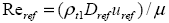
ref_mueDynamic viscosity
 at the inlet plane and mean inlet total
conditions.
at the inlet plane and mean inlet total
conditions.Note: The program identifies which of these parameters has been provided from the absolute value of the numerical input. If the value is greater than 1.0 [N s m^-2] (or equivalent value in other units), it is interpreted as a Reynolds number; if it is less than 1.0 [N s m^-2] but greater than 0.0000001 [N s m^-2], it is interpreted as the dynamic viscosity. A value of 0 causes the program to determine the dynamic viscosity from a built-in equation for the dynamic viscosity based on Sutherland’s law and the inlet total temperature. The reference Reynolds number is determined from this.
- Section 4: Fluid data (depends on value of i_fluid in .con file)
The syntax is:
cp_gas gamma_gas
if
i_fluid= 0, which indicates an ideal gas with constant specific heats, orcw_fluid rho_fluid
if
i_fluid= 1, which indicates a liquid, orR_gas gamma_gas
if
i_fluid= 2, 3, 4, or 5, which indicates a real gas with equations, orcp_gas gamma_gas z_gas
if
i_fluid= 6, which indicates a real gas with a constant real gas factor Z, orR_gas gamma_gas z_gas
if
i_fluid= 7, which indicates a real gas with a constant real gas factor Z.Parameter
Description
i_fluid= 0(ideal gas with constant specific heats)
cp_gas= Specific heat at constant pressure [J/kgK]
gamma_gas= ratio of specific heats [-] (In this document, "[-]" means dimensionless.)
i_fluid= 1(liquid)
cw_fluid= Specific heat of fluid [J/kgK]
rho_fluid= density of liquid [kg/m3]i_fluid= 2i_fluid= 3i_fluid= 4i_fluid= 5(real gas with equations)
Real gas option in which full details of the gas properties are provided in the
.rgpfile. In order to avoid changing the format of this file and internal details of the calculation, these values also need to be specified here. The values given here are estimates that are then overwritten internally in the program by the values in the real gas data file (see Specification of the Real Gas Properties Data File (*.rgp)). If no values are specified then air is assumed.R_gas= Gas constant [J/kgK]R
gamma_gas= mean ratio of specific heats [-]
i_fluid= 6(real gas with a constant real gas factor Z)
cp_gas= Specific heat at constant pressure [J/kgK]gamma_gas= ratio of specific heats [-]Z_gas= real gas factor Zpv = ZRT
i_fluid= 7(real gas with a constant real gas factor Z)
R_gas= Gas constant R [J/kgK]gamma_gas= ratio of specific heats [-]Z_gas= real gas factor Zpv = ZRT
- Section 5: Number of points on the inlet boundary where flow conditions are specified
The syntax is:
n_inbc
Parameter
Description
n_inbcNumber of points at which the inlet flow conditions are specified across the inlet plane.
Notes:
This should be less than the number of streamlines (
n_inbc<n_sl).if
n_inbc= 1 then only a single value is input and this is taken to be on the mid-streamline. Note that a single value implies that the inlet conditions have a constant total pressure, constant total temperature, and constant swirl (rcu) across the span at the inlet, whereby the value of the swirl is determined from the values specified (rcu, alpha, or cu).A maximum of 25 points is allowed.
- Section 6: Fraction of mass flow where inlet conditions are specified (n_inbc values)
The syntax is:
f_mass_inbc
Parameter
Description
f_mass_inbcn_inbcvalues of the fraction of mass along the inlet boundary at which inlet boundary conditions are specified. The first value should be 0.0 and the last value should be 1.0. Note that ifn_inbc= 1 then this has no function and a placeholder value can be specified, but this should not be omitted.- Section 7: Pressure on the inlet boundary (n_inbc values that depend on i_inbc in .con file)
The syntax is:
pt_inbc
if
i_inbc= 0.Parameter
Description
pt_inbc(
i_inbc=0)Total pressure on the inlet boundary [Pa].
Note that if an incompressible calculation is carried out it is still necessary to specify the absolute value of the total pressure on the inlet boundary.
- Section 8: Temperature on the inlet boundary (n_inbc values that depend on i_inbc in .con file)
The syntax is:
tt_inbc
if
i_inbc= 0.Parameter
Description
tt_inbc(
i_inbc= 0)Total temperature on the inlet boundary [K].
- Section 9: Swirl or angle on the inlet boundary (n_inbc values that depend on i_inbc in .con file)
The syntax is:
rcu_inbc
if
i_inbc= 0, oralpha_inbc
if
i_inbc= 1, orcu_inbc
if
i_inbc= 2.Parameter
Description
rcu_inbc(
i_inbc= 0)Swirl on the inlet boundary [m2/sec]. Note that this is the product of the local radius of the streamline and the local circumferential velocity component and is positive if the swirl is in the clockwise direction of rotation.
alpha_inbc(
i_inbc= 1)Flow angle on the inlet boundary [°]. Note that this is from the axial direction and positive in the clockwise direction of rotation.
Note also that, if a single value is specified, it is used to calculate the swirl on the mean streamline of the inlet boundary, and the swirl is then kept constant across the span. If a constant flow angle across the span is required then 2 values need to be specified across the span (
n_inbc= 2). Experience with radial turbines with high swirl at the inlet show that the specification of a single value of swirl across the span is more robust than specifying a variation of flow angle across the span.cu_inbc(
i_inbc= 2)Circumferential component of velocity [m/sec] on inlet boundary.
Note that if a single value is specified then this is used to calculate the swirl (rcu) on the mean streamline of the inlet boundary and the swirl is kept constant across the span.
- Section 10 : Aerodynamic model parameters
The syntax is:
eddy f_bl_le f_bl_te
Parameter
Description
eddySpanwise mixing parameter (eddy diffusivity).
Notes:
Typically 0.0001 to 0.001. See Streamline Curvature Throughflow Theory.
This has no function if
i_mix= 0.If
i_mix= 1 andeddy= 0.0 then a value of eddy = 0.0005 will be used.
f_bl_lef_bl_leis the meridional fraction of blade length at the leading edge where the blade is partly transparent to the flow (accounts artificially for the increased loading due to incidence). It is recommended that you specify a value of 0.0 for bothf_bl_teandf_bl_le. If bothf_bl_teandf_bl_leare equal to zero then the program estimates the values of these from the blade spacing using the equations given in Streamline Curvature Throughflow Theory. If you want, you can specify these values. If you specify 0.0 then the flow is congruent with the mean blade camber line at the leading edge. A typical value is roughly equal to the blade spacing or chord.f_bl_teFraction of blade length after which the blade is partly transparent to the flow at the trailing edge (accounts artificially for the decreased loading due to deviation as the trailing edge is approached). It is recommended that you specify a value of 0.0 for both
f_bl_teandf_bl_le. If you specify 1.0 then the flow is congruent with the mean blade camber line right up to the trailing edge. If bothf_bl_teandf_bl_leare equal to zero then the program estimates these from the blade spacing using the equations given in Streamline Curvature Throughflow Theory.
It is possible to calculate multiple operating points, in which case details of these operating points in terms of flow and speed are required in sections 11, 12, and 13.
- Section 11: Relative flow for multiple operating points (not
needed if
n_points< 2) The syntax is:
ref_point(1), ref_point(2), ref_point(3), ... ref_point(11)
Parameter
Description
ref_point(i)Flow relative to the reference flow defined in the aerodynamic file. The value
ref_mass,ref_volume, orref_phiis multiplied by the valueref_pointto determine the actual operating point.Notes:
Typically, this line consists of a list of values such as 1.15, 1.10, 1.05, 1.00, 0.95, 0.90, and 0.85, indicating 115% down to 85% of the flow at the reference point.
If the value of
i_flowis 1, the seven values listed above would be interpreted as seven different mass flows to be calculated. If the value ofi_flowis 2, the values would be interpreted as different volume flows. If the value ofi_flowis 0, the values would be interpreted as flow coefficients.The flow scales linearly with the speed, so that when operating at the 100% flow point on the 90% speed line, the flow is reduced to 90% of the reference value.
A maximum of 11 points is allowed.
- Section 12: Relative flow for multiple speed lines (not needed
if
n_speeds< 2) The syntax is:
ref_speed(1), ref_speed(2), ref_speed(3), ... ref_speed(11)
Parameter
Description
ref_speed(i)Rotational speed relative to the reference speed defined in the aerodynamic file. The value
ref_n,ref_u, orref_mach, is multiplied by the valueref_speedto determine the actual operating speed.Notes:
Typically, this section consists of a list of values such as 1.1, 1.0, 0.9, 0.8, 0.7, 0.65, 0.5.
These seven values would be interpreted as seven different speed lines to be calculated at 110%, 100%, 90%, etc., of the reference speed.
A maximum of 11 speeds is allowed.
- Section 13: Additional multiple point parameters (not needed
if
n_speeds*n_points<2) The syntax is:
map_parameter(1), map_parameter(2), ... map_parameter(11)
Parameter
Description
map_parameter(i)Not used at the moment but included to allow rules with regard to automatic map generation to be included, such as the definition of a limit in the diffusion factor to automatically provide an estimate of the stability point.
Note on Multiple operating points:
It is possible to calculate multiple operating points, in which
case details of these operating points in terms of flow and speed
are required, and sections 11, 12 and 13 provide this data. These
sections are not used if the multiple points are not calculated (n_points*n_speeds < 2 in the .con file). This option is available only for simulations
with a specified mass or volume flow and not for specified pressure
ratios.
The input data file includes sections of text lines that help you to identify the parameters defined here; see the examples in Appendix F: Examples of Correlations Data Files (*.cor). This file partly changes its structure depending on the type of correlation chosen and the number of quasi-orthogonals or blade rows being calculated. This is a complex input file, but it does not need to be changed once it is set up.
The first part of the file contains control parameters that define the layout of the remainder of the input data that is needed. The file is arranged so that it always has a standard format at the beginning (first 8 lines) but may require different data towards the end depending on the type of calculation under consideration (axial compressor, radial turbine, single stage, multistage, and so on). Similar types of simulations always use similar formats for this file, but different types of simulations may require different formats for the latter part of this file.
The file has two different structures because the specification of the empirical data relies on two different approaches.
User-specified approach
Set all of
i_loss,i_dev, andi_ewbin section 2 to a value of 1. You may specify the losses, the blockage, and deviation associated with specifically-defined quasi-orthogonals and streamlines. In the simplest and most common approach, a single value is specified on the mean streamline of the first quasi-orthogonal and this is then automatically used throughout the calculation.This approach is oriented around the quasi-orthogonals, enabling you to specify different local efficiency and blockage values for each quasi-orthogonal and streamline. Although deviation is only meaningful at the trailing edge, a similar approach, based on quasi-orthogonals, is used for deviation to be consistent with losses and blockage. In many cases, the specification of no value also allows a correlation to be used to determine the value (such as the Wiesner slip factor for a radial compressor). This approach is recommended for beginners. In general, it requires only a single value that may be changed to be specified in the correlations file. If different operating points are to be calculated, where it can be expected that the losses change, then you can take this into account by adjusting the specified loss value in the .cor file manually for each point.
Built-in correlations for losses, deviation and blockage
Set all of
i_loss,i_dev, andi_ewbin section 2 to a value of 2. You provide information that enables the program to calculate the empirical data for the losses for each blade row by selecting one of the built-in correlations, which determines the losses from the local flow field and the geometry. Different operating points will then automatically have different values of the losses.This approach is oriented around blade rows and requires data to be specified at each blade row trailing edge (or upstream of this – see later).
Note that the correlations used for individual blade rows can be changed from one blade row to another. You can also use the correlations for deviation from one source and the correlations for losses from another, if this is sensible; usually it is not sensible. In general, and for simplicity, you should apply the correlations such that all blade rows use the same correlations, and such that the losses, blockage, and deviation, are from the same source.
The correlations currently programmed can be obtained with the
use of the different parameters for i_loss_type, i_dev_type, and i_ewb_type in sections 4, 6, and 8.
Note: In some cases the same correlations can be used in slightly
different ways – this is related to the fact that the poor
description of correlations in the literature sources sometimes leads
to uncertainties in implementation. Where it is sensible different
versions have been implemented. In the machine types with many different
sources of correlations, the recommended correlation can be obtained
using values of 100, 200, 300, 400 for i_loss_type, i_dev_type, and i_ewb_type.
|
Radial Compressor Correlations |
i_loss_type / i_dev_type / i_ewb_type |
|---|---|
|
Casey-Robinson correlation |
101 / 101 / 101 |
|
Axial Compressor Correlations |
i_loss_type / i_dev_type / i_ewb_type |
|---|---|
|
Recommended correlation (203 / 203 / 201) |
200 / 200 / 200 |
|
Miller-Wright (original implementation by PCA) |
201 / 201 / 201 |
| Miller_Wright (1st revision, November 2007) |
202 / 202 / 202 |
|
Miller_Wright (2nd revision, April 2012) |
203 / 203 / 203 |
|
Axial Turbine Correlations |
i_loss_type / i_dev_type / i_ewb_type |
|---|---|
|
Recommended correlation (401 / 401 / 401) |
400 / 400 / 400 |
|
Kacker-Okapuu |
401 / 401 / 401 |
|
Dunham-Came |
402 / 402 / 402 |
If required, you can specify single values of the losses, deviation, and blockage parameters, for the first blade row or first quasi-orthogonal. These are then used throughout the domain provided that they are not changed again. In addition, it is possible to apply multiplicative and additive correction factors to the values predicted by the correlations, by the application of "fudge factors" (user-defined corrections). Generally this file does not need to be changed once it has been set up, so you might not need to understand all the intricacies of the many possibilities that it allows, and typically a standard type of correlations file can be established which can then be used for all subsequent simulations with the same set of correlations. Examples of some typical correlations data files are given in Appendix F: Examples of Correlations Data Files (*.cor), showing several specific examples for specific types of calculation.
- Section 1: Character strings identifying the correlation data (max 72 characters/line)
The syntax is:
Character string – title(1)
Character string – title(2)
Character string – title(3)
- Section 2: Integer control parameters for loss, deviation and blockage models (one line)
The syntax is:
i_loss i_dev i_ewb
Parameter
Description
i_lossDetermines the loss specification to be used.
Notes:
i_loss= 0No losses are specified and the calculation uses constant entropy. Note, however, that in order to retain similar structures for the correlations file, the lines described in sections 3 and 4 are still needed, but have no effect. This allows you to switch off the losses if necessary.
If
i_loss= 1 then a user-defined variation of efficiency, loss coefficient, or dissipation coefficient across the span is specified at the spanwise positions given in section 4. The number of positions that are defined across the span and through the domain is given in section 3. Different values of the efficiency, loss coefficient, or dissipation coefficient can be specified for different quasi-orthogonal calculating stations and spanwise positions.If
i_loss= 1, then a value on the first quasi-orthogonal is always needed. This value remains constant until changed by the next quasi-orthogonal at which the loss is defined. If only a single value is specified across the span then this is applied on the mean streamline and each streamline has the same entropy rise as on the mean streamline. If a calculation with a constant efficiency for all streamlines is required then the efficiency needs to be specified as a constant on at least two points across the span.If
i_loss= 2 then built-in loss correlations are used according to the values given in sections 3 and 4.
i_devDetermines the method for calculation of a blade outlet flow angle (deviation or slip).
Notes:
If
i_dev= 0, the flow follows the mean blade camber line given in the.geofile with no deviation. This option allows a mean S2 through-flow calculation to be carried out using the mean stream surface obtained from a series of S1 blade-to-blade calculations, provided that these are then given as the geometry of the camber surface in the.geofile. Note that, in order to retain similar structures for the correlations file, the lines described in sections 5 and 6 are still needed but have no effect.If
i_dev= 1 then data is specified in sections 5 and 6 to predict the variation of the flow angle at the blade outlet from the mean blade camber line across the span. The information can be either in the form of a deviation angle, a specified flow outlet angle, a specified slip factor, or a modification to the cosine rule, according to the type of blade row.If
i_dev= 2 then built-in correlations are used to determine the flow angle according to the type of blade row as specified in sections 5 and 6.
i_ewbDetermines the blockage correlation for boundary layers that is to be used (ewb means "end-wall blockage")
Notes:
If
i_ewb= 0 then no end-wall blockage is applied. Note that, in order to retain similar structures for the correlations file, the lines described in sections 7 and 8 are still needed, but have no effect.If
i_ewb= 1 then data is specified in sections 7 and 8 to predict the variation of the flow blockage for each quasi-orthogonal and for each streamline. A single value implies that a constant blockage value is applied in the whole calculation domain.If
i_ewb= 2 then builtin correlations are used to determine the blockage according to the type of blade row as specified in sections 7 and 8.
- Section 3: Loss input data locations
The syntax is:
n_loss_sl n_loss_qo
or
n_loss_bladerow n_dummy
If
i_lossequals 0 or 1 then the losses for each quasi-orthogonal can be specified, and the following values are required:Parameter
Description
n_loss_slNumber of the spanwise positions for which the loss data is supplied.
n_loss_qoNumber of quasi-orthogonal calculating stations through the domain on which the loss information is specified.
If
i_lossequals 2 then the losses for each blade row can be specified, and the following values are required:Parameter
Description
n_loss_bladerowNumber of separate blade rows for which the loss data is supplied.
n_dummyA placeholder integer value to ensure that section 3 always has two integer values. This enables you to switch between various alternatives without changing the structure of the data in the file.
If
i_lossequals 0 or 1, then the following version of section 4 applies:- Section 4: User-defined loss data specification (n_loss_qo * n_loss_sl lines)
This version of section 4 is applicable when
i_lossequals 0 or 1.The syntax is:
i_qo_loss k_loss f_loss loss
Parameter
Description
i_qo_lossNumber of the quasi-orthogonal calculating station on which the loss, deviation, and blockage information is specified. The specified values will be applied for all blade rows and calculating stations downstream of this quasi-orthogonal until the value is changed by a subsequent section 4 with a new value of
i_qo_loss. The first value ofi_qo_lossmust be 1. Subsequent lines may change the way in which the losses are defined.k_lossParameter to define how the losses are specified.
Notes:
If
k_loss= 1 then the small-scale static to static polytropic efficiency (eta_poly) is specified. This is used in such a way that the entropy always increases so that, for a local accelerating flow with a decrease in static enthalpy, it defines a turbine efficiency, and for a decelerating flow, it defines a compressor efficiency. This small-scale efficiency is applied in blade rows and in ducts. Note that specifying a specific value does not lead to an efficiency of the same value for the whole domain because this is dependent on both the local small-scale efficiency and the path of the process. For this,k_lossmust be set to 4 or 7. See below.If
k_loss= 2 then the entropy loss coefficient (xsi) is specified. Note that the loss coefficient is the entropy loss coefficient with respect to outlet plane dynamic head for accelerating blade rows (turbine rotors and stators) and with respect to the inlet plane dynamic head for decelerating blade rows (compressor rotors and stators). An inlet guide vane for a compressor is therefore calculated as a turbine blade row, and an outlet guide vane for a turbine as a compressor blade row. Like the deviation, this value is only used at the trailing edge of a blade row.If
k_loss= 3 then the dissipation loss coefficient (cd) is specified to determine the losses from an integration of the loss production following the so-called u-cubed model of Denton. This is applied in blade rows and in ducts.If
k_loss= 4 to 9 then various forms of efficiency are used to specify the losses, as follows:k_loss = 4 total-total polytropic efficiency
k_loss = 5 total-static polytropic efficiency
k_loss = 6 static-static polytropic efficiency
k_loss = 7 total-total isentropic efficiency
k_loss = 8 total-static isentropic efficiency
k_loss = 9 static-static isentropic efficiency
These are applied in blade rows and in duct regions.
In duct regions, these values are applied to the change from one quasi-orthogonal to the next. Clearly if the total enthalpy does not change, the use of 4 or 7, which give a total-total efficiency, is meaningless. In blade rows the full range is allowed, but options 6 and 9 are probably not very relevant. Use of 5 and 8 is not recommended because specifying a total-static efficiency that is too high may lead to a total-total efficiency that is greater than unity.
Option 4 or 7 is now recommended for rotor blade rows. This change forces the impeller total-total efficiency to be exactly the value that is specified. It is more robust, especially with real gas equations, because only the velocity triangle at the impeller outlet is involved in the estimate of the losses, and there is no need to use the real gas equations at each point in the stage when determining the entropy. It also has the advantage that the losses become exactly as specified, which was not the case with the option using a small-scale local polytropic efficiency.
If
k_loss= 10 then the loss in a stator vane can be specified as a total pressure loss coefficient.If
k_loss= 11 then the performance of a stator vane can be specified as a static pressure rise coefficient.These options have been programmed so that different blade rows may have different values of
k_loss.
f_lossThe fraction of the span at which the value of loss applies. If only a single value is given, it is applied at the mean streamline independent of the value of
f_loss.lossDepending on the value of
k_loss, this is interpreted as a small-scale polytropic efficiency (etapol), a loss coefficient (xsi), a dissipation coefficient (cd), or other items given.If
i_lossequals 2 then the following version of section 4 applies:- Section 4: Correlation-based loss data specification (n_loss_bladerow lines)
This version of section 4 is applicable when
i_lossequals 2.The syntax (of a single line) is:
i_loss_bladerow i_loss_type factor1 factor2 factor3 factor4 factor5 factor6
Parameter
Description
i_loss_bladerowNumber of the blade row on which the loss information is specified. The specified values will be applied for all blade rows downstream of this blade row until the value is changed by a subsequent section 4 with a new value of
i_loss_bladerow, and then this will again be applied until changed. The first value must be 1.i_loss_typeParameter to define which correlations are used for the blade row losses. The current loss correlations incorporated into the method are as follows:
Radial Compressor Correlations
i_loss_type= 101Casey-Robinson correlation
Axial Compressor Correlations
i_loss_type= 200Recommended correlation (203)
i_loss_type= 201Miller_Wright (original implementation by PCA) 201
i_loss_type= 202Miller_Wright (1st revision, November 2007)
i_loss_type= 203Miller_Wright (2nd revision, April 2012)
Axial Turbine Correlations
i_loss_type= 400Recommended correlation (401)
i_loss_type= 401Kacker-Okapuu
i_loss_type= 402Dunham-Came
factor_loss1 tofactor_loss6User-defined multiplication or addition factors to the losses determined by the correlations. This allows the loss correlations to be modified to improve matching with experimental or CFD data. These have different functions for the different correlation systems. In the case of the Cox-Casey correlations these provide some empirical constants for the models used.
i_loss_type= 11: Casey-Robinson radial compressor model.Factor 1: Impeller total-total efficiency at design point (eta_d)
Factor 2: Design tip-speed Mach number (Mu2_d)
Factor 3: Design flow coefficient (phi_d)
Factor 4: Type of stage: 1.0 = turbocharger, -1.0 = process
Factor 5: Type of diffuser: 1.0 = vaned, -1.0 =vaneless
Factor 6: not in use
i_loss_type= 21, 22, 23, 24, 41, and 42: Factors on losses.Factor 1: Multiplication factor on profile losses
Factor 2: Multiplication factor on secondary losses
Factor 3: Multiplication factor on tip clearance losses
Factor 4: Multiplication of penetration of secondary losses
Factor 5: Multiplication of penetration of tip clearance losses
Factor 6: Not in use
These are all generally specified as a value of 1.0.
i_loss_type= 31: Cox-Casey radial turbine model.Factor 1: Small-scale polytropic efficiency
Factor 2: Loss multiplier for tip clearance loss vortex
Factor 3: Loss penetration of tip clearance vortex (fraction of span from the tip)
Factors 4 to 6: Not in use
- Section 5: Deviation input data locations
The syntax is:
n_dev_sl n_dev_qo
or
n_dev_bladerow n_dummy
If
i_devequals 0 or 1 then the deviation for each quasi-orthogonal can be specified, and the following values are required:Parameter
Description
n_dev_slNumber of spanwise positions for which the flow angle data is supplied.
n_dev_qoNumber of quasi-orthogonal calculating stations on which the flow angle information is specified.
If
i_devequals 2 then the deviation flow angle data can be specified for each blade row, and the following values are required:Parameter
Description
n_dev_bladerowNumber of separate blade rows for which the flow angle data is supplied.
n_dummyA placeholder integer value to ensure that section 5 always has two integer values.
If
i_devequals 0 or 1 then the deviation for each quasi-orthogonal can be specified, and the following version of section 6 is applicable:- Section 6: Flow angle data specification (n_dev_qo * n_dev_sl lines)
This version of section 6 is applicable when
i_devequals 0 or 1.The syntax is:
i_qo_dev k_dev f_dev dev
Parameter
Description
i_qo_devNumber of the quasi-orthogonal calculating station on which the deviation information is specified. The specified values will be applied for all blade row trailing edges downstream of this quasi-orthogonal until the value is changed by a subsequent section 6 with a new value of
i_qo_dev. The first value must be 1.k_devDetermines the type of outlet flow angle calculation, as follows:
If
k_dev= 1 then the deviation angle is specified (in degrees).If
k_dev= 2 then the relative outlet flow angle is specified (in degrees).If
k_dev= 3 then a slip factor is specified and applied on the mean line (dimensionless). Note that if no value is specified then the Wiesner slip factor is used. Only recommended for radial impellers and not for mixed flow stages, which should use deviation.If
k_dev= 4 then a slip factor is applied at each radius of the trailing edge (dimensionless). Note that if no value is specified then the Wiesner slip factor is used. Only recommended for radial impellers and not for mixed flow stages, which should use deviation.If
k_dev= 5, this is analogous tok_dev= 3, but the slip factor correlation of Xuwen Qiu is applied on the mean-line.If
k_dev= 6, this is analogous tok_dev= 4, but the slip factor correlation of Xuwen Qiu is applied on each streamline separately.
f_devThe fraction of the span of at which the value of the deviation (and similar things) applies. If only a single value is given, it is applied at the mean streamline independent of its value.
devDepending on the value of
k_dev, this is interpreted as a deviation angle, flow angle, slip factor, or correction to the cosine rule.If
i_devequals 2 then the deviation for each blade row can be specified, and the following version of section 6 is applicable:- Section 6: Flow angle data specification (n_dev_bladerow lines)
This version of section 6 is applicable when
i_devequals 2.The syntax is:
i_bladerow_dev i_dev_type factor1 factor2 factor3 factor4 factor5 factor6
Parameter
Description
i_bladerow_devNumber of the blade row on which the deviation information is specified. The specified values will be applied for all blade row trailing edges downstream of this quasi-orthogonal until the value is changed by a subsequent section 6 with a new value of
i_bladerow_dev. The first value must be 1.i_dev_typeParameter to define which correlations are used for the blade row deviations. The current deviation correlations incorporated into the method are as follows:
Radial Compressor Correlations
i_dev_type= 101Casey-Robinson correlation
Axial Compressor Correlations
i_dev_type= 200Recommended correlation (203)
i_dev_type= 201Miller-Wright (original implementation by PCA)
i_dev_type= 202Miller_Wright (1st revision, November 2007)
i_dev_type= 203Miller_Wright (2nd revision, April 2012)
Axial Turbine Correlations
i_dev_type= 400Recommended correlation (401)
i_dev_type= 401Kacker-Okapuu
i_dev_type= 402Dunham-Came
More General Correlations
i_dev_type= 501User defined on a blade row by blade row basis
i_dev_type= 502Carter’s rule
i_dev_type= 503Cosine rule (Taupel)
factor_dev1 tofactor_dev6User-defined coefficients or addition factors to the deviations determined by the correlations. This allows the deviation correlations to be modified to improve matching with experimental or CFD data.
i_dev_type= 11: Casey-Robinson radial compressor model.Factor 1: Impeller slip factor for rotors. If this is specified as 0.0 then the Wiesner slip factor is used.
Factor 1: Deviation angle for stators. If this is specified as 0.0 then Carter’s rule is used.
Factors 2 to 6: Not in use.
i_dev_type= 21, 22, 23, 24: Correction to deviation.Compressor deviation correlations of Miller and Wright for DCA compressor blades with modifications.
Factor 1: Additive factor in degrees (°) on hub deviation
Factor 2: Additive factor in degrees (°) on mean deviation
Factor 3: Additive factor in degrees (°) on tip deviation
Factors 4 to 6: Not in use.
Typically values of 0.0 would be used.
i_loss_type= 31: Graham Cox radial turbine model.Factor 1: Shroud deviation angle offset (d_s). If specified as 0.0 then 10.0° is used.
Secondary deviation parameters for the hub:
Factor 2: Hub related vortex swirl (half) amplitude (Amp_h). If specified as 0.0 then 3.0 is used.
Factor 3: Hub related vortex swirl variation 1/4 wavelength (QW-h). If 0.0 is specified then 0.34 is used.
Secondary deviation parameters for the shroud:
Factor 4: Shroud related vortex swirl (half) amplitude (Amp_s). If 0.0 is specified then 6.0 is used.
Factor 5: Shroud related vortex center (VC s). If 0.0 is specified then 0.86 is used.
Factor 6: Hub trailing edge thickness parameter. If specified as less than 0.07 then 0.26 is used, otherwise 0.16 is used.
For details see publication of Cox. Note that values of 0.0 for all parameters is acceptable.
i_dev_type= 41 or 42: Kacker-Okapuu, Dunham-Came.Turbine deviation using the cosine rule.
These have different functions for the different correlation systems. In the case of the Cox-Casey correlations these provide some empirical constants for the models used. Otherwise generally as follows.
Factor 1: Additive factor in degrees (°) on hub deviation.
Factor 2: Additive factor in degrees (°) on mean deviation.
Factor 3: Additive factor in degrees (°) on tip deviation.
Factor 4: Not in use.
Factor 5: Not in use.
Factor 6: Not in use.
- Section 7: Blockage input data locations
The syntax is:
n_ewb_sl n_ewb_qo
or
n_ewb_bladerow n_dummy
If
i_ewbequals 0 or 1 then the blockage for each quasi-orthogonal can be specified, and the following values are required:Parameter
Description
n_ewb_slNumber of spanwise positions for which the blockage data is supplied.
n_ewb_qoNumber of quasi-orthogonal calculating stations on which the blockage information is specified.
If
i_ewbequals 2 then the blockage correlation can be specified for each blade row, and the following values are required:Parameter
Description
n_ewb_bladerowNumber of separate blade rows for which the blockage is supplied.
n_dummyA placeholder integer value to ensure that section 7 always has two integer values.
If
i_ewbequals 0 or 1 then the blockage for each quasi-orthogonal can be specified, and the following version of section 8 is applicable:- Section 8: End wall blockage data specification (n_dev_qo * n_dev_sl lines)
This version of section 8 is applicable when
i_ewbequals 0 or 1.The syntax is:
i_qo_ewb k_ewb f_ewb ewb
Parameter
Description
i_qo_ewbNumber of the quasi-orthogonal calculating station on which the blockage information is specified. The specified values will be applied for all blade rows and calculating stations downstream of this quasi-orthogonal until the value is changed by a subsequent section 4 with a new value of
j_qo_ewb. The first value must be 1.k_ewbDetermines the type of blockage calculation. Has no effect because the blockage is input in only one form as below.
f_ewbThe spanwise location of the value of the blockage. If only a single value is given, it is applied at all streamlines.
ewbEnd-wall boundary layer blockage is specified. A value of 0.05 represents 5% blockage of the flow channel by the end-wall boundary layers. If zero is specified then there is no end-wall boundary layer blockage. Typically a constant value is specified across the whole span, but this parameter can be varied across the span to allow for the higher blockage in the end-walls related to blade ends with tip clearance.
If
i_ewbequals 2 then the blockage for each blade row can be specified, and the following version of section 8 is applicable:- Section 8: End wall blockage data specification (n_ewb_bladerow lines)
This version of section 8 is applicable when
i_ewbequals 2.The syntax is:
i_bladerow_ewb i_ewb_type factor1 factor2 factor3 factor4 factor5 factor6
Parameter
Description
i_bladerow_ewbNumber of the blade row on which the blockage information is specified. The specified values will be applied for all blade row trailing edges downstream of this quasi-orthogonal until the value is changed by a subsequent section 6 with a new value of
i_bladerow_ewb. The first value must be 1.i_ewb_typeParameter to define which correlations are used for the blade-row blockage. Currently only axial compressor blockage correlations based on the Miller-Wright calculations are incorporated into the method as follows:
i_ewb_type= 200Recommended (202)
i_ewb_type= 201Blockage calculated using the Miller Wright method adjusted to allow the blockage to vary through the blade row. The blockage value, however, is not used.
i_ewb_type= 202Blockage calculated as in
i_ewb_type= 201. The calculated values are used. The calculation leads to different values of blockage at all quasi-orthogonals and is based on a throughflow interpretation of the Miller Wright method.i_ewb_type= 203Blockage calculated and not used. The value of the blockage is calculated at trailing edges only and then remains constant to the next trailing edge. This is done to be consistent with SC90C blockage calculations, which are based on a ductflow interpretation of the Miller Wright method.
factor_ewb1 tofactor_ewb6User-defined multiplication or addition factors to the blockage determined by the correlations. This allows the end-wall blockage correlations to be modified to improve matching with experimental or CFD data. These have different functions for the different correlation systems.
Factor 1: Not in use.
Factor 2: Not in use.
Factor 3: Not in use.
Factor 4: Not in use.
Factor 5: Not in use.
Factor 6: Not in use.
The real gas property input data file includes lines of text
that help you to identify the parameters defined there. The name .rgp is used to describe this file, but the content
is different compared to the usual (Ansys CFX) real gas property file,
which has a similar name.
An example of a real gas property data file is given in Appendix H: Example of a Real Gas Property Data File (*.rgp).
- Section 1: Character strings identifying the aerodynamic data (max 72 characters/line)
The syntax is:
Character string - title(1)
Character string - title(2)
Character string - title(3)
- Section 2: Name of gas (72 characters)
The syntax is:
gas_name
Parameter
Description
gas_nameText characters defining the gas name
- Section 3: Molecular mass and/or Gas constant
The syntax is:
MW Gas_R
Parameter
Description
MWMolecular mass of gas (kg/kmol)
Gas_RGas constant = Universal gas constant/MW J(kg/K)
Note that if either of these values is specified with a numerical value of less than 0.1 then it is calculated from the universal gas constant using the other value, which needs to be specified correctly.
- Section 4: Critical point parameters and acentric factor
The syntax is:
Pc (Pa) Tc (K) Vc (m3/kg) gas_omega (-)
Parameter
Description
PcCritical pressure (Pa)
TcCritical temperature (K)
VcSpecific volume at critical point (m3/kg)
gas_omegaAcentric factor (-)
- Section 5: Temperature limits of specific heat curve polynomial
The syntax is:
T_min (K) T_max(K) order_T_poly (max 8)
Parameter
Description
T_minLowest temperature in range (K)
T_maxHighest temperature in range (K)
n_T_coeffnumber of coefficients = Order of polynomial plus 1
- Section 6: Coefficients of cp polynomial (T_min < T < T_max)
The syntax is:
A1 A2 A3 A4 A5 A6 A7 A8
Parameter
Description
A1First coefficient in polynomial
A2Second coefficient in polynomial
…Subsequent coefficients
A8Eighth coefficient in polynomial
Note that this representation only allows a single interval dependent polynomial to be defined. If a third order polynomial is specified then only four coefficients are needed.
Note that if the value of the first coefficient specified is less than the value of the gas constant then all of the coefficients will be multiplied by the gas constant as in some databases this form of the coefficients is used.
The output data file includes lines of text in ASCII format that show the results of the simulation. The file consists of several sections:
- Section 1: Input data
At the start of this file, a list of the input data files that were used is recorded in this file so that a record of the file names is available.
INPUT DATA FILES: Control data file: agard.con Geometric data file: agard.geo Aerodynamic data file: agard.aer Correlation data file: agard.cor Restart data file: agard.rst OUTPUT DATA FILES: Results file: agard.out Tecplot data file: impeller.txt CFD-POST data file: agard.csv Convergence history file: agard.hst Interface output file: agard.int- Section 2: Reference data
The program uses the input data to set up the values of various other parameters; for example, where the reference mass flow is specified, the reference volume flow is calculated. The values of all other parameters not included in the input specification are given in this section. In addition, the internal calculation of the damping factors is provided. Other data listed here relates to the program's own estimates of the throat area and the throat position. An example is given below.
Example radial compressor calculation:
Reference flow parameters ------------------------- Mass flow distribution across streamlines: 0.000 0.062 0.125 0.188 0.250 0.312 0.375 0.438 0.500 0.562 0.625 0.688 0.750 0.812 0.875 0.938 1.000 Inlet distribution across streamlines: Fraction of flow: 0.00 Total pressure: 100000.00 Total temperature: 293.00 Inlet swirl: 0.00 Ideal gas calculation gamma_gas gas_m r_gas cp_gas 1.400 3.500 287.200 1005.200 ref_pt(bar) ref_tt ref_rhot ref_soundt 1.0000 293.00 1.1884 343.23 Reference rotational direction: clockwise ref_d ref_u ref_omega ref_n 0.2700 398.10 2948.91 28160.0 ref_mach ref_phi ref_mass ref_volume 1.1599 0.0667 2.3000 1.94 ref_re ref_mue 6963614.0 0.00001834 ref_n1 ref_n2 ref_n3 28160.0 0.0 0.0 Simulation with no spanwise mixing Iterate to mass flow, ref_mass = 2.30000 First approximation of streamline positions taken from an earlier calculation Estimated max. thicknesses for blade row 1 span 0.00000 0.17343 0.34429 0.51305 0.67879 0.84126 0.97669 1.00000 thickne 0.00351 0.00319 0.00291 0.00266 0.00241 0.00215 0.00195 0.00191 User-input throat widths for blade row 1 span 0.00000 0.17343 0.34429 0.51305 0.67879 0.84126 0.97669 1.00000 throat 0.01760 0.02137 0.02460 0.02732 0.02959 0.03141 0.03257 0.03276 Estimated throat positions for blade row 1 span 0.00000 0.17343 0.34429 0.51305 0.67879 0.84126 0.97669 1.00000 throat_pos 0.00969 0.02084 0.03424 0.04835 0.06224 0.07573 0.08688 0.08882 Empirical correlation data User specified losses User specified deviation No blockage specified Relaxation factor calculation of Wilkinson ------------------------------------------ Maximum aspect ratio: 6.0667 at calculating station: 5 damp_sc (user input): 0.2500 damp_sc (Wilkinson): 0.0577 Warning: damp_sc reduced by the code to the value suggested by Wilkinson- Section 3: Short history of the convergence
The
.outfile contains a statement about convergence of the results. A converged calculation includes a header such as the following:*********************************************** * VistaTF converged -it_main: 6 * * * * cm_error(%) p_error(%) mass_error(%) * * 0.042 0.000 0.000 * *********************************************** * Global performance * * * * mass (kg/s): 0.093200 * * est. choke: 0.107995 * * t-t t-s s-s * * eta_p: 0.8453 0.7415 * * eta_s: 0.8553 0.7583 * * pr: 0.5800 0.5374 0.6100 * * er (1/pr): 1.7243 1.8609 1.6392 * * power (kW): -5.4316 * ***********************************************
A more detailed convergence history is output to the history file, which is described in Specification of Convergence History Data File (*.hst).
- Section 4 : Simulation results on quasi-orthogonal planes and streamlines
Results are provided at every quasi-orthogonal requested (see control file parameter
i_print_plane) in the level of detail requested (parameteri_print_level). The data is provided across the span for each streamline. If the number of streamlines is greater than 9 then data for every second streamline is given. The structure of this data and the information provided varies depending on the type of calculation station. The example below is for a radial impeller leading edge:Quasi-orthogonal - i = 3 n_blade n_curve i_type i_row i_spool 13 6 3 0 0 Rotor blade - leading edge At throat (or just upstream of throat) Compressor Radial impeller Throat area = 0.00274713 Annulus choke parameters: dm_dcm = 0.79601 Mach_eff = 0.45166 choke mass at this q_o = 7.72100 choke_mass of machine = 7.72100 choke_mass of this blade row = 7.72100 current_mass at this q_o = 6.70000 inlet mass flow = 6.70000 Factor on slope of ree: grad_re = 1.00000 cm_guess_save = 152.57564 Flow parameters - print_level=1 streamline 1 3 5 7 9 11 13 15 17 r [m] 0.07612 0.08753 0.09759 0.10647 0.11445 0.12176 0.12855 0.13493 0.14100 z [m] -0.13500-0.13500-0.13500-0.13500-0.13500-0.13500-0.13500-0.13500-0.13500 1/rc[1/m] -5.996 1.353 2.758 2.818 2.475 1.984 1.438 0.864 0.244 throat mm 23.00 24.41 25.66 26.77 27.40 27.84 28.17 28.30 29.00 f_sl [-] 0.17503 0.17777 0.18110 0.18431 0.18734 0.19021 0.19295 0.19556 0.19806 f_qo [-] 0.00000 0.17593 0.33098 0.46775 0.59076 0.70340 0.80807 0.90652 1.00000 f_bl [-] 0.00000 0.00000 0.00000 0.00000 0.00000 0.00000 0.00000 0.00000 0.00000 f_thr [-] 0.02584 0.03400 0.04157 0.04823 0.05408 0.05923 0.06379 0.06785 0.07150 gamma_in 1.00000 1.00000 1.00000 1.00000 1.00000 1.00000 1.00000 1.00000 1.00000 gamma_out 0.00000 0.00000 0.00000 0.00000 0.00000 0.00000 0.00000 0.00000 0.00000 cm [m/s] 146.87 142.25 145.30 149.18 152.57 155.22 157.11 158.32 158.87 - error % 0.0001 -0.0002 0.0001 0.0001 0.0001 0.0001 0.0000 -0.0002 -0.0001 - max 169.57 166.48 168.30 172.19 174.87 177.33 179.61 180.96 186.11 cu [m/s] 0.00 0.00 0.00 0.00 0.00 0.00 0.00 0.00 0.00 M_cm [-] 0.437 0.423 0.432 0.444 0.455 0.463 0.469 0.472 0.474 M_crit[-] 1.000 1.000 1.000 1.000 1.000 1.000 1.000 1.000 1.000 M_rel [-] 0.765 0.837 0.914 0.985 1.050 1.109 1.163 1.213 1.260 beta_fl° -55.19 -59.65 -61.79 -63.21 -64.34 -65.33 -66.23 -67.08 -67.90 beta_bl° -43.03 -46.77 -50.17 -52.99 -55.37 -57.46 -59.30 -60.92 -62.35 incidence 12.16 12.88 11.62 10.22 8.98 7.86 6.93 6.16 5.55 p [bar] 0.8706 0.8778 0.8730 0.8669 0.8614 0.8571 0.8540 0.8519 0.8510 t [K] 282.38 283.04 282.60 282.04 281.54 281.14 280.84 280.66 280.57 rho[kg/m3] 1.0742 1.0806 1.0764 1.0710 1.0661 1.0623 1.0595 1.0577 1.0569 A*/A 0.9485 0.9758 0.9935 0.9998 0.9980 0.9907 0.9799 0.9666 0.9517 m/m_max 0.8661 0.8545 0.8633 0.8664 0.8725 0.8753 0.8747 0.8749 0.8536 m_prime 75.46 84.55 95.91 106.88 116.97 126.15 134.46 141.98 148.76 m_pr_max 87.12 98.94 111.09 123.37 134.07 144.11 153.70 162.27 174.26 ch_ratio 0.8662 0.8545 0.8634 0.8664 0.8725 0.8753 0.8748 0.8749 0.8537 Flow parameters - print_level=2 eps [°] 12.82 14.30 12.54 10.34 8.13 6.01 4.00 2.08 0.23 psi [°] 77.18 75.70 77.46 79.66 81.87 83.99 86.00 87.92 89.77 c [m/s] 146.87 142.25 145.30 149.18 152.57 155.22 157.11 158.32 158.87 w [m/s] 257.28 281.50 307.34 330.98 352.35 371.83 389.80 406.55 422.31 u [m/s] 211.24 242.91 270.83 295.46 317.60 337.88 356.73 374.45 391.29 wu [m/s] -211.24 -242.91 -270.83 -295.46 -317.60 -337.88 -356.73 -374.45 -391.29 M_abs [-] 0.437 0.423 0.432 0.444 0.455 0.463 0.469 0.472 0.474 alpha_fl° 0.00 0.00 0.00 0.00 0.00 0.00 0.00 0.00 0.00 pt [bar] 0.9921 0.9921 0.9921 0.9921 0.9921 0.9921 0.9921 0.9921 0.9921 tt [K] 293.00 293.00 293.00 293.00 293.00 293.00 293.00 293.00 293.00 s [J/kgK] 2.29 2.29 2.29 2.29 2.29 2.29 2.29 2.29 2.29 ds[J/kgK] 0.00 0.00 0.00 0.00 0.00 0.00 0.00 0.00 0.00 ewb [-] 0.0500 0.0500 0.0500 0.0500 0.0500 0.0500 0.0500 0.0500 0.0500 Loading parameters - print_level=3 w_s [m/s] 287.34 314.82 342.24 366.60 388.17 407.50 425.12 441.51 456.87 w_p [m/s] 227.21 248.18 272.45 295.36 316.53 336.16 354.47 371.59 387.74 M_ws [-] 0.855 0.936 1.018 1.091 1.157 1.215 1.268 1.318 1.364 M_wp [-] 0.676 0.738 0.810 0.879 0.943 1.002 1.058 1.109 1.157 C_btob [-] 0.234 0.237 0.227 0.215 0.203 0.192 0.181 0.172 0.164
The text data file includes lines of text in ASCII format that
are intended as input for various software packages for producing
plots of the converged results. The text files can be used as input
data for Tecplot. Standard layout (.lay)
files for Tecplot have been prepared which allow typical diagrams
to be produced on the basis of this data. The information is structured
in such a way that it can just as easily be used by Excel or some
other similar program with an appropriate interface.
In fact, after running the program, several standard .txt files for Tecplot are produced: one covering the
whole flow field and one for each blade row. The flow field data is
written in the file prefix.txt, and the blade-row
data in the files row_01_prefix.txt, row_02_prefix.txt, and so on, whereby the number of
the files refers to the blade rows numbered from the start of the
computational domain. You only need to provide the name of one of
these files in the vista_tf.fil file, because
the others are automatically generated and numbered by the program.
Some standard Tecplot layout files have been prepared that operate
on the .txt files to produce typical plots
that are needed during the design of a component. For example, the
files used for radial compressor impellers are called: flowfield_2d_v_2_0.lay and rc_impeller_row1.lay. The first of these prepares a plot showing the 2D meridional channel
with contours of constant parameters (such as meridional velocity,
swirl velocity, static temperature, Mach number, cm_error and so on) and the second prepares blade loading plots for a typical
blade row. The layout file (.lay) determines
the format of the plot and the ASCII .txt file contains the data to be plotted. The format and the scales
can also be changed on-line within Tecplot by clicking on the screen.
Other Layout files for other cases (ac = axial compressor, hp = hydraulic
pump, ht= hydraulic turbine, rt = radial turbine, at= axial turbine)
are also available and these can be easily customized (scales, parameters
and so on).
The standard Tecplot layout files (.lay) have all been written to work on the data in text files named impeller.txt and row_01_impeller.txt, and so on. The first dataset, impeller.txt, contains information for the contour plots showing the meridional
velocity and other parameters projected on the meridional plane and
the second, row_01_impeller.txt, contains
the various blade loading parameters for an individual blade row.
If the case concerned has several blade rows then there is also a
file called row_02_impeller.txt, row_03_impeller.txt, and so on; there is one file for
each blade row. A new layout file is needed for each blade row. The
letters "impeller" in this name rely on the fact that
the prefix for the .txt file has this name
in the vista_tf.fil file.
Other prefixes will produce .txt files
containing the prefix as specified in the vista_tf.fil file. In this case, the layout files need to be modified; the layout
files can be opened in a text editor; the name of the .txt file is on the second line. This name can then
be changed to match the name given as a prefix in the vista_tf.fil file. Alternatively, the same layout files
can be used for several cases if all data that needs to be plotted
always retains the prefix name impeller;
the text output file from vista_tf always
has the name impeller.txt in the vista_tf.fil file.
Generally, a good strategy is to set up the .aero, .cor, .con, and .txt files with a certain prefix in the vista_tf file and to let these keep the same names for
all runs on a particular case because they normally do not change
as the design progresses. It then remains necessary to switch the .geo files around to look at different impellers, or
else the prefix for the .geo file can be
retained and the cases can be distinguished by simply putting them
into different directories to distinguish the different cases.
The data in the prefix.txt file is
in approximately the following format:
TITLE
Flow field data for whole flow field from hub to shroud for all q-os

Variables = '"r" "z" "cm" "cu" "cr" "cz" "p" "t" "pt" "tt" "s" "h" "q_o" "error" "choke_ratio"
"M_rel" "M_abs" "alpha_flow" "beta_flow" "1/rc" "beta"'

"r"                  Radius coordinate
"z"                  Axial coordinate
"cm"                 Meridional velocity
"cu"                 Swirl velocity
"cr"                 Radial velocity
"cz"                 Axial velocity
"p"                  Static pressure
"t"                  Static temperature
"pt"                 Total pressure
"tt"                 Total temperature
"s"                  Entropy
"h"                  Static enthalpy
"q_o"                an integer identifying the particular type of q-o
"error"              Meridional velocity error in %
"choke_ratio"        choke ratio (ratio of local mass flow to choke flow at this location)
"M_rel"              Relative Mach number
"M_abs"              Absolute Mach number
"alpha_flow"         Absolute flow angle [°]
"beta_flow"          Relative flow angle [°]
"1/rc"               Curvature ( inverse of the radium of curvature)
"beta"               Blade angle [°]
The data in the row_01_prefix.txt file
is approximately in the following format:
TITLE
Data on hub, mean and tip streamlines for all blade rows from LE to TE
and data along leading edge and trailing edge of all blade rows

VARIABLES =VARIABLES = "i_type", "f_bl", "M", "M_s", "M_p", "w", "w_s", "w_p",...
"p", "p_s", "p_p", "c_btob", "c_htos", "beta_bl", "beta_fl", "dep_angle", "gamma_in", ...
gamma_out", "f_qo", "de_haller", "cp_ideal", "incidence", "deviation", "lambda", ...
"df_lieblein", "zweifel" "c_lift", "c_zw"
"f_bl"               Fraction of meridional distance along the blade
"M"                  Mean mid-passage Mach number (relative to blade)
"M_s"                Suction side Mach number
"M_p"                Pressure side Mach number
"w"                  Mean mid-passage velocity (relative to blade)
"w_s"                Suction surface velocity
"w_p"                Pressure surface velocity
"p"                  Static pressure in mid-channel between two blades
"p_s"                Suction surface static pressure
"p_p"                Pressure surface static pressure
"c_btob"             Blade to blade loading parameter
                     (c_btob = (w_s-w_p)/w, that is the difference between suction surface
                     and pressure surface velocities divided by the mid-channel velocity
"c_htos"             Hub to shroud loading parameter
                     (c_htos = (cm_shroud – cm_hub)/ cm_mean, that is the difference
                     between the meridional velocity on the casing and the hub divided by
                     the mean velocity.
"beta_bl"            Blade angle in degrees [°]
"beta_fl"            Flow angle in degrees [°]
"dep_angle"          Departure angle in degrees [°]
"gamma_in"           Blending function at blade inlet
"gamma_out"          Blending function at blade outlet
"f_qo"               fractional distance along q-o
"de_haller"          De Haller number
                     (de_haller = w2/w1, that is outlet/ inlet relative velocity
"cp_ideal"           Ideal static pressure recovery coefficient
                     ( Cpideal = 1 – (de_haller)**2 )
"incidence"          Incidence at the leading edge [°]
"deviation"          Deviation at the trailing edge[°]
"lambda"             Work coefficient ( lambda = (h2-h1)/u**2, that is Deltah / u squared)
"df_lieblein"        Lieblein Diffusion Factor (see below)
"zweifel"            Zweifel loading parameter (see below)
"c_lift"             Lift coefficient (see below)
"c_zw"               Lift coefficient times solidity (see below)
Note that the values of the last four parameters have been included mainly for axial blade rows. Each of them includes the blade solidity (ratio of chord to spacing) in its definition. In radial machines, the spacing and solidity change with radius along the streamline. There is no generally agreed method to calculate these parameters for radial machines, so the mean value of the spacing has been selected in the following definitions used in Vista TF. In any case, caution is suggested in the use of these parameters for radial machine blade rows because the experimental basis for limit values has generally been derived from axial machines.
Lieblein diffusion factor (df_lieblein)
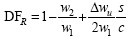
Zweifel coefficient (zw)
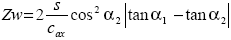
Lift coefficient (CL)
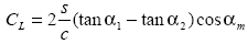
where 
Zweifel number (c_zw)
The text data files *prefix.csv include
lines of text in ASCII Comma Separated Variable format. These files
contain user surface data for CFD-Post, and are intended as input
for CFD-Post for plotting purposes. For details on the user surface
data format for CFD-Post, see USER SURFACE Data Format in the CFD-Post User's Guide.
In the current .csv files, the following
data is available for each grid node:
[Name]
Vista-TF
[Data]
X [m], Y [m], Z [m], Cm [m/s], Cu [m/s], Cr [m/s], Cz [m/s], p [bar], t [K], s [J kg^-1 K^-1],
h [J/kg], q_o [], error [], M_rel[], M_abs[], rc [m^-1]
The file global_prefix.csv contains
a list of parameters, whereby these are specified as:
Name 1 = value1 [units]
Name 2 = value2 [units]
Separated by comment lines which begin with "#".
In addition, there are four additional files produced for each blade row from 1 to n:
row_0n_hub_prefix.csv
row_0n_mean_prefix.csv
row_0n_tip_prefix.csv
row_0n_loading_prefix.csv
These contain essentially similar information to the row_0n_prefix.txt files described above, but this is
split into four separate files: one for the hub, one for the mean
span, one for the tip, and one for the loading parameters.
The convergence history data file includes lines of text in ASCII format that show the convergence of the simulation. This contains details of the convergence of the main iterative procedures, and extensive details of the terms in the radial equilibrium equation for each stream tube and calculating plane. It is rare for this to be examined in any depth, but this can be useful to identify problems if the solution fails to converge.
- Section1: Input Data
At the start of the
.hstfile, the input data is recorded. This is essentially in the same format as the input files. At the start of this file, there is a list of the names of the input data files that were used. This information can be useful if an error occurs in the input data because the.hstfile records only the data that has been successfully read into the program.- Section 2: Convergence Data
At every iteration, a summary of the iteration progress is provided. It looks like this:
History of the main iteration loop ---------------------------------- it_main: 1 error_cm(%): 100.000 at i_qo: 0 j_sl: 0 it_mass: 11 at i_qo: 1 it_main: 2 error_cm(%): 38.940 at i_qo:10 j_sl:17 it_mass: 11 at i_qo: 1 it_main: 3 error_cm(%): 30.036 at i_qo:10 j_sl:17 it_mass: 11 at i_qo: 3 it_main: 4 error_cm(%): 24.600 at i_qo:10 j_sl:17 it_mass: 11 at i_qo: 4 it_main: 5 error_cm(%): 20.939 at i_qo:10 j_sl:17 it_mass: 11 at i_qo: 5 it_main: 6 error_cm(%): 18.306 at i_qo:10 j_sl:17 it_mass: 11 at i_qo: 6 it_main: 7 error_cm(%): 16.403 at i_qo:10 j_sl:17 it_mass: 11 at i_qo: 6 ..... it_main: 284 error_cm(%): 0.013 at i_qo: 7 j_sl:17 it_mass: 1 at i_qo: 1 it_main: 285 error_cm(%): 0.012 at i_qo: 7 j_sl:17 it_mass: 1 at i_qo: 1 it_main: 286 error_cm(%): 0.011 at i_qo: 7 j_sl:17 it_mass: 1 at i_qo: 1 it_main: 287 error_cm(%): 0.010 at i_qo: 7 j_sl:17 it_mass: 1 at i_qo: 1 it_main: 288 error_cm(%): 0.009 at i_qo: 7 j_sl:17 it_mass: 1 at i_qo: 1- Section 3: Streamline Curvature Solution Data
At every quasi-orthogonal, details of the terms in the radial equilibrium equation for each stream tube are provided. This can be useful in identifying errors and also helpful to determine the magnitude of the terms in the equations. "rhs" is the value of the right hand side of the radial equilibrium equation, giving the square of the gradient of the meridional velocity.
The streamline curvature solution data looks like this:
Quasi-orthogonal - i = 5
 n_blade n_curve i_type i_row i_spool
    9       8       3      0     0
Radial equilibrium parameters -print_level = 4
rhs          1049.90 1059.86  871.10  684.48  510.68  349.39  199.63   55.28
ret             0.00    0.00    0.00    0.00    0.00    0.00    0.00    0.00
ret_dh          0.00    0.00    0.00    0.00    0.00    0.00    0.00    0.00
ret_tds         0.00    0.00    0.00    0.00    0.00    0.00    0.00    0.00
ret_drcu        0.00    0.00    0.00    0.00    0.00    0.00    0.00    0.00
sct          1049.90 1059.86  871.10  684.48  510.68  349.39  199.63   55.28
sct_rc        641.48  681.97  558.43  431.70  315.91  211.42  118.25   34.87
sct_dcm       408.43  377.89  312.67  252.78  194.78  137.97   81.38   20.40
bft             0.00    0.00    0.00    0.00    0.00    0.00    0.00    0.00
dft             0.00    0.00    0.00    0.00    0.00    0.00    0.00    0.00
cm_error%    -0.0010  0.0002 -0.0003 -0.0007 -0.0007 -0.0003  0.0003  0.0010
f_mixing      0.0000  0.0000  0.0000  0.0000  0.0000  0.0000  0.0000  0.0000
1/rc       2.853   4.466   4.153   3.505   2.773   2.016   1.261   0.517  -0.209
cm       137.936 145.590 152.396 157.708 161.716 164.594 166.473 167.450 167.568
rcu        0.000   0.000   0.000   0.000   0.000   0.000   0.000   0.000   0.000
drcu/dm   47.323  53.336  48.562  35.419  15.376 -11.226 -43.868 -81.313-123.649
s          1.885   1.885   1.885   1.885   1.885   1.885   1.885   1.885   1.885
bl_block   0.0000  0.0000  0.0000  0.0000  0.0000  0.0000  0.0000  0.0000  0.0000