


This tutorial includes:
- 2.1. Overview of the Mesh Creation Process
- 2.2. Preparing the Working Directory
- 2.3. Defining the Geometry
- 2.4. Creating the Topology and Mesh
- 2.5. Reviewing the Mesh Data Settings
- 2.6. Reviewing the Mesh Quality on the Hub and Shroud Tip Layers
- 2.7. Looking at Mesh Data Values
- 2.8. Analyzing the Mesh Quality
- 2.9. Visualizing the Hub-to-Shroud Element Distribution
- 2.10. Observing the Shroud Tip Mesh
- 2.11. Examining the Mesh Qualitatively
- 2.12. Creating a Legend
- 2.13. Saving the Mesh
- 2.14. Saving the State (Optional)
This tutorial demonstrates the basic workflow for generating a CFD mesh using Ansys TurboGrid. As you work through this tutorial, you will create a mesh for a blade passage of an axial compressor blade row. A typical blade passage is shown by the black outline in the figure below.
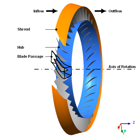
The blade row contains 36 blades that revolve about the negative Z axis. A clearance gap exists between the blades and the shroud, with a width of 2.5% of the total span. Within the blade passage, the maximum diameter of the shroud is approximately 51 cm.
You will save the mesh in a format that can be used by Ansys CFX in a CFD simulation.
If this is the first tutorial you are working with, it is important to review Introduction to the Ansys TurboGrid Tutorials before beginning.
Before Ansys TurboGrid can create a mesh, you must provide it with several pieces of information. Such information includes the location of the geometry files (hub, shroud, and blades), the mesh topology type, and the distribution of mesh nodes. All of the data that you provide is stored in a set of data objects known as CCL objects.
The Ansys TurboGrid user interface organizes the CCL objects in a tree view known as the object selector. You can use the object selector to select and edit the CCL objects; the objects are listed from top to bottom in the standard order for creating a mesh. The user interface also has a toolbar for selecting and editing the CCL objects; the icons are arranged from left to right in the standard order for creating a mesh.
Regardless of whether you use the object selector or the toolbar, you should generally follow this sequence when creating a mesh:
Define the geometry by loading files and changing settings as required.
Optionally choose a topology method, then unsuspend the
Topology Setobject if necessary.Optionally modify the
Mesh Datasettings that govern the number and the distribution of nodes in various parts of the mesh.If you plan to make a fine (high-resolution) mesh, you can optionally set the mesh density at a later time in order to minimize processing time while establishing other aspects of the mesh. Note that changing the mesh density can affect the mesh quality.
Optionally add intermediate 2D layers that guide the 3D mesh in the spanwise direction. By default, layers are added as required when you generate the topology or the 3D mesh.
Check the mesh quality. As required, make adjustments to the
Mesh Datasettings and the number and distribution of layers.Save the mesh and state as required.
Create a working directory.
Ansys TurboGrid uses a working directory as the default location for loading and saving files for a particular session or project.
Download the
rotor37.zipfile here .Unzip
rotor37.zipto your working directory.Ensure that the following tutorial input files are in your working directory:
BladeGen.inf
profile.curve
hub.curve
shroud.curve
Set the working directory and start Ansys TurboGrid.
For details, see Setting the Working Directory and Starting Ansys TurboGrid.
The provided geometry files, which consist of a BladeGen.inf file plus three curve files, were created
using BladeGen. To load the information contained in those files,
you will load the BladeGen.inf file. Ansys TurboGrid uses
this file to set the axis of rotation, the number of blades, and a
length unit that characterizes the scale of the machine. It also uses
this file to identify the curve files, which it then loads to define
the curvature of the hub, shroud, and a single blade. The geometric
data from the input files is processed to generate a geometric representation,
an outline of which appears in the viewer.
After the geometry has been generated, you are invited to browse
through the objects created under the Geometry object in the object selector.
Initially, the blades extend from the hub to the shroud. After inspecting the geometry, you will create the required gap between the blade and the shroud.
Load the BladeGen.inf file:
Click File > Load TurboGrid Init File.
Open
BladeGen.inffrom the working directory.The progress bar at the bottom right of the screen shows the geometry generation progress. After the geometry has been generated, the viewer in the Mesh workspace shows the hub, shroud, and blade for one passage. Along the blade, you can see the leading and trailing edge curves (green and red lines, respectively). An outline drawing (the
Outlineobject) traces the 3D space that is available for meshing; the latter consists of an inlet domain, passage, and outlet domain. In this tutorial, you will generate a mesh for the passage only.Note: It is possible to adjust the upstream and downstream extents of the hub and shroud surfaces (by changing the
InletandOutletgeometry objects). It is also possible to create an extended mesh that includes the inlet and outlet domains (by editing theMesh Datasettings).
Examine the geometry in the 3D Viewer:
In the Mesh workspace, toggle the visibility check box next to each object in the object selector and observe the change in the viewer.
Note the correlation between the geometry objects listed in the object selector and the locations in the geometry.
In order to avoid cluttering the view, ensure that the visibility is turned on only for these objects:
Hub,Shroud,Blade 1,Outline.
Examine and set the machine type:
Open
Geometry>Machine Datafrom the object selector by double-clickingMachine Datain the object selector, or by right-clickingMachine Dataand selecting Edit from the shortcut menu that appears.Here you can see basic information about the geometry. Note that the units specified for
Base Unitsrepresent the scale of the geometry being meshed; these units are not used for importing geometric data nor do they govern the units written to a mesh file; they are used for the internal representation of the geometry to minimize computer round-off errors.Set Machine Type to
Axial Compressor.Setting the machine type helps TurboGrid choose appropriate topology templates later in the mesh creation process.
Click Apply.
Examine the hub:
Open
Geometry>Hub.Here you can see information about which file was used for hub data and how the file was interpreted. Similar information can be seen by opening the
ShroudandBlade 1objects. Note that, for theHubandShroudobjects, the Curve Type parameter is set toPiece-wise linear; this is a result of loading aBladeGen.inffile.Click Display all blade instances
 to obtain a view of the entire geometry.
Click Display single blade instance
 to show a single blade instance once again.
To complete the geometry, create a small gap between the blade and the shroud. The blade should be shortened to 97.5% of its original span because the gap width, as specified in the problem description, is 2.5% of the total span.
Open
Geometry>Blade Set>Shroud Tip.Set Tip Option to
Constant Span.Set Span to
0.975.Click Apply.
The names of the objects in the Geometry branch of the object selector are shown in black non-italic text,
indicating that the Geometry objects are all
defined. This completes the geometry definition.
The Topology Set object is initially suspended in order to save
computational effort while defining the geometry. When you unsuspend the
Topology Set object, the remaining computations are performed,
resulting in a 3D mesh.
Right-click
Topology Setand turn off Suspend Object Updates.The
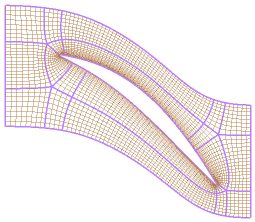
Topology Setobject name in the object selector changes to black non-italic text, indicating that this object is generated. The topology appears on the hub and shroud as a structure of thick lines. Thinner lines show where individual mesh elements are located.The 3D mesh is also generated. The number of nodes and elements are displayed at the bottom left.
Change the view to clearly show the topology on the hub:
Click Hide all geometry objects
 .
.Turn on the visibility of
Layers>Hubto show the topology on the hub.Click Hide all mesh objects
 .
.Right-click a blank area in the viewer, and click Predefined Camera > View From +X from the shortcut menu.
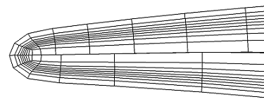
The heavy lines in Figure 2.1: ATM Topology and 2D Mesh on the Hub indicate the topology lines; the thinner lines show the 2D mesh for the hub.
The Mesh Data settings control the number
and distribution of mesh elements.
Open
Mesh Data.Note that Method is set to
Global Size Factorand Size Factor is set to1.In the status bar in the bottom-left corner of Ansys TurboGrid, you can see that the number of mesh nodes is on the order of 200000.
Layers are constant-span surfaces. You can display the topology on a layer. You have already
seen the hub layer in Figure 2.1: ATM Topology and 2D Mesh on the Hub. At this point, there are two
layers: Layers > Hub, and Layers >
Shroud Tip.
If the topology were grossly skewed or distorted on the hub or shroud tip layer, the
Layers object would be shown with red text in the object selector.
Now the topology is defined and the mesh quality is acceptable on all layers.
The mesh is generated automatically after the Layers object is processed.
Later in this tutorial, you will check 3D mesh measures and inspect the mesh visually.
The Mesh Data editor tabs display information about the mesh. In the following
steps, you will examine the number and distribution of elements from
hub to shroud tip and from shroud tip to shroud.
Open
Mesh Data.Click the Passage tab.
Look in the Spanwise Blade Distribution Parameters frame. Method is set to
Proportionalwith a factor of1.0. The other boxes in the frame are disabled, but show the current value for each option that Ansys TurboGrid has calculated.You can see that # of Elements is
25.Click the Shroud Tip tab.
Look in the Shroud Tip Distribution Parameters frame. Method is set to
Match Expansion
at Blade Tip
. You can see that the number of elements from shroud tip to shroud is 16.
3D mesh measures are available.
These are analogous to the 2D mesh measures that are calculated on
layers. As for the 2D mesh measures, the 3D mesh measures have quality
criteria set in the Mesh Analysis > Mesh Limits object.
Mesh measures of some mesh elements may fall outside the criteria.
When any mesh measure fails to meet the criteria, Mesh Analysis
(Error) > Mesh Statistics (Error) will
appear in red text in the object selector. You can open Mesh Analysis (Error) to display the Mesh Statistics dialog box. In the Mesh Statistics dialog box,
you can select one of the items in red and click Display to see the locations in the mesh where the statistics fail to meet
the corresponding criterion.
Not all of the mesh measures carry the same importance. For
example, it is necessary to have a mesh with no negative volumes.
Generally, poor angles should also be fixed, but the
Element Volume Ratio and Edge Length
Ratio values should be judged based on your requirements.
Check the 3D mesh statistics:
For a visual frame of reference, ensure that
Layers>HubandLayers>Shroud Tipare visible.Open
Mesh AnalysisorMesh Analysis>Mesh Statistics.The Mesh Statistics dialog box appears, and shows that the mesh statistics are acceptable based on the current quality criteria.
Close the Mesh Statistics dialog box.
To demonstrate the use of the 3D Mesh visualization
objects, look at the mesh distribution from hub to shroud as follows:
Click Unhide geometry objects
 .
.Turn off the visibility of the following objects:
Geometry>Blade Set>Blade 1Layers>HubLayers>Shroud Tip
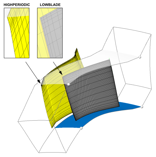
Turn on the visibility of the following objects under
3D Mesh:HIGHPERIODIC.LOWBLADE GEO HIGHLOWBLADE GEO LOW
Observe the element distribution from hub to shroud tip and from shroud tip to shroud.
See Figure 2.2: Hub-to-Shroud Element Distribution.
A mesh interface exists in the shroud tip gap. In order to see this interface:
Turn on the visibility of
3D Mesh>SHROUD TIP.Click Hide all geometry objects
.Zoom in to view the mesh on the shroud tip.
Figure 2.3: Surface Group: Tip Near Trailing Edge shows this mesh at the trailing edge of the blade. Note how the nodes do not line up along the middle of the blade, due to the default use of a general grid (GGI) interface along the shroud tip of the blade.
Turn off the visibility of
3D Mesh>SHROUD TIP.Click Unhide geometry objects
.
You will now examine the mesh qualitatively using a turbo surface.
Change the Show Mesh turbo surface so that it
appears on the hub, and color it to show the variation in Edge Length Ratio (a variable that was computed at the
time the mesh was generated):
Turn on the visibility of
3D Mesh>Show Mesh.Open
3D Mesh>Show Mesh.Leave Variable set to
K.Kis equal to the node number in the spanwise direction, ranging from 1 at the hub to a positive integer value at the shroud.Set Value to
1.This will cause the turbo surface to appear on the hub.
Click the Color tab.
Set Mode to
Variable.Set Variable to
Edge Length Ratio.Set Range to
Local.This will cause the range of colors in the color map to be distributed over the range of values found on the turbo surface, rather that over the global range or a user-defined range.
Click the Render tab.
Ensure that Draw Faces is selected.
Click Apply.
To avoid visual conflicts between the turbo surface and the hub, which are coincident, turn off the visibility of
Geometry>Hub.
Note that you can edit the rendering properties of the hub to
achieve a similar result. The advantage of using a turbo surface is
that you can redefine its location. For example, you could change
the value of K in the current turbo surface to
see Edge Length Ratio on a different nodal plane.
Note: You can create new turbo surfaces. To begin the process of creating a new turbo surface, click Insert > User Defined > Turbo Surface.
Note: To show distinct color bands, you could make a contour plot object that applies to an existing locator (geometric surface, turbo surface, or other graphic objects that involve surfaces). To begin the process of creating a contour plot, ensure that you have a suitable locator already defined, then click Insert > User Defined > Contour.
Tip: For objects that are colored by a variable, it is best to view them with lighting turned off so that the colors are not altered according to the angle of view. The lighting is controlled by a setting on the Render tab.
In the previous section, you modified a turbo surface by coloring
it according to Edge Length Ratio. To reveal
the color map used to match values of Edge Length Ratio with particular colors, create a legend for the turbo surface:
Click Insert > User Defined > Legend.
Click to accept the default name.
Set Plot to
TURBO SURFACE:Show Mesh.Set Title Mode to
Variable and Location.Click Apply.
A legend appears in the viewer, showing the correspondence between values of
Edge Length Ratioand colors for theShow Meshobject.
You may want to modify 3D Mesh > Show Mesh to plot it on different locations, or to color
it by different variables. The legend will be updated automatically
whenever you make changes to the turbo surface.
Save the mesh:
Click File > Save Mesh As.
Ensure that Files of type is set to
Ansys CFX Mesh Files.Set Export Units to
cm.Set File name to
rotor37.gtm.Ensure that your working directory is set correctly.
Click Save.