Automatic meshing in Ansys Forte uses on-the-fly Cartesian volume mesh generation combined with immersed boundary method. Mesh update intervals are controlled by a combination of the following input parameters and constraints:
Time Interval: Mesh will be updated if the elapsed time since the previous mesh update is exceeding this user-specified time interval.
Rotation/Crank Angle Interval: The mesh update interval is controlled to be approximately equivalent to this angle interval. This angle is with respect to the rotation motion of the highest RPM in the simulation system, including both slider-crank motion (piston motion in IC engine cases), simple rotation, and planetary motion (including both primary rotation and secondary rotation).
Flow Travel Distance: This distance threshold is used to limit the mesh update interval to be sufficiently small such that the distance the flow with the largest velocity magnitude can travel between two consecutive mesh updates will not exceed this threshold.
Spray Particle Travel Distance: This distance threshold is used to limit the mesh update interval to be sufficiently small such that the distance the fastest-traveling spray particle can travel between two consecutive mesh updates will not exceed this threshold.
Flame Propagation Distance: This distance threshold is used to limit the mesh update interval to be sufficiently small such that the distance the fastest-traveling flame can propagate between two consecutive mesh updates will not exceed this threshold.
When Automatic Meshing is indicated, the Mesh Controls tree contains two sub-nodes for required input: Material Point and Global Mesh Size.
Material Point: This is a point that is inside the cylinder throughout the cycle and that enables the automatic mesh generation to stay within the boundaries. You must set this point appropriately before the automatic meshing can work properly.
Note: The Material Point must be located in a position that is always inside the geometry during the entire cycle and is at least one unit cell length away from any boundaries.
Global Mesh Size: Affects meshing and refinement throughout the system.
In addition to the controls described above, the Mesh Controls icon bar (as well as right-clicking the Mesh Controls node on the Workflow tree) provides icons that can be used to create additional mesh-size constraints.
Each of the mesh-size controls can be specified as static (Always active) or dynamic (active only During specified time or crank-angle intervals) with a reference to a relative time frame (see Time Frames). For example, refinement in the squish region near a moving piston boundary may only be necessary when the piston is near top-dead-center (TDC) position. For simulation of a full cycle, this may mean setting two controls for the two intervals (for example, 350 to 370 CA, 710 to 730 CA) during the cycle of a 4-stroke engine while the squish region is most active. However, near the valve seat, mesh refinement must Always be set to 1/4 or finer.
If the mesh-size controls are active During Crank Angle Interval, you can select the Crank Angle Option as Cyclic or Global. The Cyclic option is helpful in specifying controls that are repetitive in a multi-engine-cycle simulation. In this case, the user-supplied crank angle values will be converted to fit in the range of [0, 720) °CA (for 4-stroke engines) or [0, 360) °CA (for 2-stroke engines). The activation interval will then be treated as cyclic and repeated on a 720-degree schedule (4-stroke) or 360-degree schedule (2-stroke). You may choose to Use Global Crank Angle Limits to impose a global crank angle range for the cyclic repetition, beyond which mesh-size controls are not active. If the Crank Angle Option is Global, no cyclic conversion is applied to the user-supplied crank angle values.
Point Refinement Depth
 : A Point Refinement is a sphere of mesh-size influence, where you
specify the minimum size for a cell edge within that sphere, relative to the Global Mesh Size,
the location of the point at the center of the sphere, and the radius of the sphere in
absolute physical units. These parameters are entered in the Point Refinement Editor panel
after a new control is created. Since you can have multiple points of refinement, you can name
each control for reference purposes and it will appear with that name in the Mesh Controls
list.
: A Point Refinement is a sphere of mesh-size influence, where you
specify the minimum size for a cell edge within that sphere, relative to the Global Mesh Size,
the location of the point at the center of the sphere, and the radius of the sphere in
absolute physical units. These parameters are entered in the Point Refinement Editor panel
after a new control is created. Since you can have multiple points of refinement, you can name
each control for reference purposes and it will appear with that name in the Mesh Controls
list.Surface Refinement Depth
 : Surface refinement allows you to specify a mesh-size constraint at any
surface defined in the geometry, such as an inlet or valve surface. The Editor panel includes
specification of the minimum size relative to the Global Mesh Size, as well as selection of
one or more boundaries at which the size constraint will apply.
: Surface refinement allows you to specify a mesh-size constraint at any
surface defined in the geometry, such as an inlet or valve surface. The Editor panel includes
specification of the minimum size relative to the Global Mesh Size, as well as selection of
one or more boundaries at which the size constraint will apply.Feature Refinement Depth
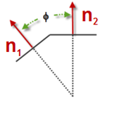
 : Feature refinement allows you to specify a mesh-size constraint to be
applied along edges whose feature angle is greater than a specified feature-angle threshold
value. The Editor panel includes specification of the feature angle and a distance away from
the feature angle to apply the refinement. Feature angle (φ) is defined as the angle
between the two adjacent faces along an edge
: Feature refinement allows you to specify a mesh-size constraint to be
applied along edges whose feature angle is greater than a specified feature-angle threshold
value. The Editor panel includes specification of the feature angle and a distance away from
the feature angle to apply the refinement. Feature angle (φ) is defined as the angle
between the two adjacent faces along an edge  (see Figure 3.12: Feature Refinement Depth diagram illustrating phi).
Line Refinement Depth
 : Line refinement allows you to specify a mesh-size constraint along any
line in the geometry. The Editor panel includes specification of the minimum size relative to
the Global Mesh Size, as well as selection of one or more boundaries at which the size
constraint will apply.
: Line refinement allows you to specify a mesh-size constraint along any
line in the geometry. The Editor panel includes specification of the minimum size relative to
the Global Mesh Size, as well as selection of one or more boundaries at which the size
constraint will apply.Gap Feature Refinement Control and Gap Resistance Model
 : Gap feature refinement allows you to identify a small gap formed by two
surfaces where you can specify mesh refinement and apply certain model options within the gap.
: Gap feature refinement allows you to identify a small gap formed by two
surfaces where you can specify mesh refinement and apply certain model options within the gap. Each gap definition must select exactly two surfaces as its Location. Fluid cells residing in the gap region will be marked as gap cells based on two gap detection criteria (see below). Each gap cell will be assigned a gap size value based on the closest gap distance between the two selected surfaces.
Note: The gap size value is one of the variables reported as spatially resolved solutions (see Table 3.6: Spatially resolved variables that are output to the solution file when Gap Feature Refinement Control is used in Spatially Resolved Panel).
The two gap detection criteria are:
Surface Proximity is used as a distance criterion for identifying the gap region. Specifically, a fluid region will be identified as a gap if the distance between the two nearby surfaces is smaller than the Surface Proximity value. The recommended value for setting the Surface Proximity is to use the automatic option called Determine from Surface Depth.
If you choose to specify the Surface Proximity manually, the guideline is that it should be equal to or slightly larger than the local volume mesh size near the surfaces that form the gap, after considering the surface depth mesh refinement applied to the surfaces and before considering the gap feature mesh refinement. Note that in the automatic determination option, the value is automatically set to be equal to the local surface depth refinement at the gap × a 1.1 factor.
The Surface Alignment Threshold controls the angular deviation allowed between the faces defining the gap in the gap region detection. A value of zero indicates the faces bounding a gap must be parallel, a higher value is more permissive and will detect more cells. Its default setting is 45 degrees and it should work for most cases.
Mesh refinement: Once the gap region is identified by Forte, it will apply mesh refinement according to the gap feature refinement control. Specifically, set the Size as Fraction of Global Size to determine the mesh size used in the gap region, which is a fraction of the global mesh size.
In certain industrial applications, geometric gap sizes between the two surfaces can be very small. Resolving them would require micron-level fluid cells and incur impractical computational cost. In such situations, Forte does not rely on using micron-level tiny cells to resolve the gaps. When setting up Forte's simulation, the Cartesian cells in the gap region can be larger than the local gap size. Even if the mesh resolution in the gaps is refined relative to the global mesh size, it can be coarser than the local gap size, to control computational cost. But in this case, we recommend that you Enable Gap Model to accurately model the flow physics in the gap region.
Gap resistance model: If the local mesh size is larger than the geometric gap size, you can Enable Gap Model to model the higher flow resistance caused by the smaller geometric gap sizes. The gap resistance model is formulated based on the analytical solution of a shear flow between two parallel plates. The gap resistance factor is defined as the ratio of decelerated velocity and the original velocity:

(3–1)
where Cshear is the shear constant (its value is 12 based on the parallel-plate shear flow model),
 is the geometric gap size,
  is the kinematic viscosity, and
  is the CFD time step. The gap model applies a resistance force term to the
flow field, causing the flow field to decelerate. The formula shows the impact of the gap
model on the flow velocity after the current time step.
is the CFD time step. The gap model applies a resistance force term to the
flow field, causing the flow field to decelerate. The formula shows the impact of the gap
model on the flow velocity after the current time step. The gap resistance will always try to decelerate the flow, which is why fgap is always < 1. But meanwhile, the pressure gradient term in the flow equation tries to accelerate the flow
As mentioned earlier, the geometric gap size is measured by the distance between the two surfaces forming the gap. In some special cases where the geometric gap size is not the same as the real gap size, the Gap Size Scale Factor can be used to scale the measured gap sizes to match their "real" physical values. The scaled gap size, computed as h=geometric gap size × gap size scale factor, is then used as the input for the gap resistance model.
Note: The Gap Size Scale Factor is applied only within the gap resistance model. It does not affect the gap cell identification or the gap size values reported in spatially resolved solutions.
The Block Flow Across Gap option in the gap model allows the flow leakage across the gap zone to be minimized. If the gap is associated with a built-in FSI or System Coupling FSI, the blockage will be applied only when the moving body of the FSI is inactive, that is, when its displacement is below the activation threshold. It is recommended that the blockage be turned on for gaps associated with FSI. For gaps not associated with FSI, it is typically unnecessary to turn on this blockage option. Note that this flow blockage option cannot completely block the flow. It can only mitigate the leakage through the gap as much as possible.
Ansys does not have formal and dedicated documentation regarding validation of the gap model, but see this case study using City University's screw compressor, and a paper that presents the simulation of a claw-shaped gas pump using Ansys Forte [33], [16], [18].
Secondary Volume
 : Creates a Secondary-Volume-based mesh control in the Workflow tree for
specifying a multiplier to the mesh size to a selected sub-volume. For more inforhmation about
sub-volume and how to specify it, refer to Sub-Volumes.
This mesh control allows you to use a mesh size different from the global mesh size in the
sub-volume. You may set the mesh size smaller than the global mesh size to get finer mesh
resolution in the sub-volume. Alternatively, you can set a mesh size larger than the global
mesh size, which may be useful in allowing certain regions of the domain to remain coarse when
refinement is not needed. For example, in an engine simulation, it allows keeping the port
region coarse when valves are closed.
: Creates a Secondary-Volume-based mesh control in the Workflow tree for
specifying a multiplier to the mesh size to a selected sub-volume. For more inforhmation about
sub-volume and how to specify it, refer to Sub-Volumes.
This mesh control allows you to use a mesh size different from the global mesh size in the
sub-volume. You may set the mesh size smaller than the global mesh size to get finer mesh
resolution in the sub-volume. Alternatively, you can set a mesh size larger than the global
mesh size, which may be useful in allowing certain regions of the domain to remain coarse when
refinement is not needed. For example, in an engine simulation, it allows keeping the port
region coarse when valves are closed.Solution Adaptive Meshing
 : Solution adaptive meshing allows refining the mesh based on a solution
field (or gradient) at the current time step. Both a solution field and selection criteria
must be specified. Cells meeting the selected criteria will be refined one level per mesh
update, up to the maximum depth specified in the control. Previously refined cells that no
longer meet the criteria will be coarsened one level per mesh update, up to the default cell
depth, unless influenced by another control. Three types of criteria are available:
: Solution adaptive meshing allows refining the mesh based on a solution
field (or gradient) at the current time step. Both a solution field and selection criteria
must be specified. Cells meeting the selected criteria will be refined one level per mesh
update, up to the maximum depth specified in the control. Previously refined cells that no
longer meet the criteria will be coarsened one level per mesh update, up to the default cell
depth, unless influenced by another control. Three types of criteria are available:This will target cells whose field value lies beyond a user-specified statistical significance of the bulk fluid value, given as a multiple of the standard deviation (sigma) of the field or gradient average:
low_threshold = field_average + sigma_threshold * sigma
Cells whose field or gradient value is greater than low_threshold and less than high_threshold will be targeted for refinement. This approach is especially useful when applied to gradients. A sigma threshold value between 0.5 and 1.0 is recommended. A lower value lowers the threshold used to target cells and therefore leads to more refinement, while a higher value raises the threshold and results in less refinement.
Percentage of current solution bounds
This will target cells whose field value lies within the user-specified range, where the range is defined as described in this table:
minimum value of the selected field or gradient at the current time step
maximum value of the selected field or gradient at the current time-step
Cells whose field or gradient value is greater than low_threshold and less than high_threshold will be targeted for refinement. Note this criterion is currently unavailable when a species field or gradient is selected.
This allows expressing the range of values used to target cells directly. Cells whose field or gradient value is greater than the given lower bound and less than the given upper bound will be targeted for refinement.