This tutorial describes how to use Ansys Forte CFD to simulate combustion in a port-injected spark ignition internal combustion engine with moving valves. Engine geometry is imported and Ansys Forte's automatic mesh generation is used to create the computational mesh on-the-fly during the simulation.
The files for this tutorial are obtained by downloading the
siengine_pfi_automesh.zip file
here
.
Unzip siengine_pfi_automesh.zip to your working folder.
SIEngine_Sample.stl : This is the geometry file.
ExhaustLift.csv and IntakeLift.csv: Two files of data describing the intake and exhaust valve lifts. Profiles such as these can be imported (from .csv files) or manually entered in the Profile Editor.
Spatial_Output_CAs.csv : Specifies when spatially resolved data such as velocity, temperature, species concentrations, etc., will be output.
SIEngine_PortInjected_AMG_Tutorial.ftsim: A project file of the completed tutorial, for verification or comparison of your progress in the tutorial set-up.
The sample files are provided as a download. You have the opportunity to select the location for the files when you download and uncompress the sample files.
Note: This tutorial is based on a fully configured sample project that contains the tutorial project settings. The description provided here covers the key points of the project set-up but is not intended to explain every parameter setting in the project. The project files have all custom and default parameters already configured; the text highlights only the significant points of the tutorial.
Forte may be launched in a command line mode to perform certain tasks such as preparing a run for execution, importing project settings from a text file, or various other tasks described in the Forte User's Guide. One of these tools allows exporting a textual representation of the project data to a text file.
Example
forte.sh CLI -project <project_name>.ftsim -export tutorial_settings.txt
Briefly, you can double-check project settings by saving your project and then running the command-line utility to export the settings in your tutorial project (<project_name>.ftsim), and then use the command a second time to export the settings in the provided final version of the tutorial. Compare them with your favorite diff tool, such as DIFFzilla. If all the parameters are in agreement, you have set up the project successfully. If there are differences, you can go back into the tutorial set-up, re-read the tutorial instructions, and change the setting of interest.
The port-fuel injection is approximated by a premixed, pre-vaporized blend of fuel and air in the intake port. There are two exhaust and intake valves and the simulation domain includes the intake and exhaust manifolds (Figure 5.1: Port-injected engine geometry with valves and ports defined ). In other words, the initialization of the gas composition is used to specify the fuel-air mixture in the intake-port region and perfect mixing within the port is assumed. The case is reacting flow, with a single component, 59-species single-component fuel that is appropriate for engine simulations that are not concerned with knock. See the Ansys Forte User Guide for details of the chemistry.
The project setup workflow follows the top-down order of the workflow tree in the Ansys Forte Simulate interface. The components irrelevant to the present project will not be mentioned in this document, and you can simply skip them and use the default model options.
Note: All Editor panel options that are not explicitly mentioned in this tutorial should be left at their default values. Changed values on any Editor panel do not take effect until you press the Apply button. Always press the Apply button after modifying a value, before moving to a new panel or the Workflow tree.
This tutorial involves importing an existing geometry into Ansys Forte and
setting up the automatic mesh generation using a global mesh size and adapting the mesh near the
valves. To import the geometry, go to the Workflow tree and click Geometry. This opens the
Geometry icon bar. Click the Import Geometry ![]() icon. In the resulting dialog, pull down and select Surfaces from
one or more STL files. In the dialog that opens with STL file import options, accept
the defaults.
icon. In the resulting dialog, pull down and select Surfaces from
one or more STL files. In the dialog that opens with STL file import options, accept
the defaults.
The mesh will be automatically generated during the simulations. When the file browser launches, navigate to the folder Tutorial_SIENGINE_PFI_Automesh then select SIEngine_sample.stl. Note that once you have imported the geometry, there are a number of actions that you can perform on the items in the Geometry node, such as scale, rename, transform, invert normals, or delete geometry elements.
The Geometry imports in an opaque mode and possibly preset zoom level.
It is often helpful to Refit ![]() the view or use the mouse wheel to re-zoom. To change opacity, right-click
the Geometry node in the Workflow tree and select Medium for the
Opacity level of all geometry elements, as shown in Figure 5.1: Port-injected engine geometry with valves and ports defined
.
the view or use the mouse wheel to re-zoom. To change opacity, right-click
the Geometry node in the Workflow tree and select Medium for the
Opacity level of all geometry elements, as shown in Figure 5.1: Port-injected engine geometry with valves and ports defined
.
Subvolumes are useful to refine regions of interest, such as the chamber. The subvolume can then be used in the mesh controls to control the size of the mesh in the selected subvolume. On the Workflow tree, right-click the Geometry > Sub-Volumes node to create a subvolume named Sub-Volume-Cylinder. For Location, select the following surfaces to define the subvolume: Head, Liner, and Piston. For the Material point, accept the default Reference Frame using the Global Origin. Set the Location using Cartesian Coord. System to X = 0, Y = 0 and Z = 1.0 cm. Click Apply.
The Material Point is the point in the domain that tells Ansys Forte where the mesh will be generated and should be located at least one unit cell length away from any boundaries. This point must be inside of the domain throughout the entire simulation. Typically it is located near the head so it is still inside the domain at TDC.
Mesh Controls > Material Point: Accept the default Reference Frame using the Global Origin. Set the Location using Cartesian Coord. System to X = 0, Y = 0 and Z = 1.0 cm. Click Apply.
From the Workflow tree, use Mesh Controls > Global Mesh Size to set the global Mesh Size to 0.2 cm.
Note: This is the recommended mesh size; a coarser setting of 0.3 cm could be used for tutorial purposes to produce a shorter runtime.
Set the Small Feature Deactivation Factor to 0.5.
Next, you will refine the mesh around key geometric features such as valves and the piston, walls, and open boundaries ("continuative outflows"). The following steps show how the mesh is refined for key geometric features. From the Mesh Controls node, you can add Point, Surface, Line, or Feature Refinements, or Small Feature Avoidance Controls. Ansys recommends the following general practices for setting mesh refinement in a full-cycle 4-stroke engine simulation that includes ports and valves:
Refinement at Wall Boundaries. Use ½ the global mesh size where the mesh intersects with the wall boundaries. An extended layer of refinement is added by default to ensure that the refinement includes a full layer when the Cartesian mesh intersects curved or slanted boundaries.
Surface Refinement: Click the Mesh Controls node in the Workflow tree. In the icon bar, click the New Surface Refinement
 icon and name the new control AllWalls. (This
indicates that along the selected surfaces, cells of this smaller size and greater
refinement will be used.) A new AllWalls item appears under Mesh Controls in the Workflow
tree. In the panel that appears, select all of the items in the Location list, except be
sure to exclude the Pressure_In and Pressure_Out open-boundary surfaces (refinement will be
set up along these surfaces separately). Be sure the list’s scroll bar is showing to
ensure all the list items are displayed. Accept the default mesh Size as Fraction
of Global Size as ½. Set the Number of Cell Layers to Extend
Refinement from Surface to 1. Keep the default of
Active to Always in the drop-down list below the
refinement-layer entry. Click Apply. An initial refinement is applied
over all wall boundaries with a ½ Size Fraction of Global
Size.
icon and name the new control AllWalls. (This
indicates that along the selected surfaces, cells of this smaller size and greater
refinement will be used.) A new AllWalls item appears under Mesh Controls in the Workflow
tree. In the panel that appears, select all of the items in the Location list, except be
sure to exclude the Pressure_In and Pressure_Out open-boundary surfaces (refinement will be
set up along these surfaces separately). Be sure the list’s scroll bar is showing to
ensure all the list items are displayed. Accept the default mesh Size as Fraction
of Global Size as ½. Set the Number of Cell Layers to Extend
Refinement from Surface to 1. Keep the default of
Active to Always in the drop-down list below the
refinement-layer entry. Click Apply. An initial refinement is applied
over all wall boundaries with a ½ Size Fraction of Global
Size.
Refinement at Open Boundaries (Continuative Outflows). Again, the continuative outflows will use ½ the global mesh size, but use 2 extended layers of refinement, to make sure the continuative outflows have smooth refinement where the inlet intersects walls.
In the Mesh Controls icon bar, click the New Surface Refinement
icon and name the new control OpenBoundaries. In
the panel that appears, select all of the open-boundary surfaces (the
Pressure_In and Pressure_Out boundary surfaces)
from the Location list. Accept the default mesh Size as
Fraction of Global Size as 1/2. Set the Number of
Cell Layers to Extend Refinement from Surface to 2. Click
Apply. An initial refinement control is applied over all wall
boundaries with a ½ Size Fraction of Global Size.
Refinement Around the Valve Stems. Here we want to make sure we have smaller cells in the regions around the valve stems, where velocities will be greatest during intake and exhaust portions of the cycle.
In the Mesh Controls icon bar, click the New Surface Refinement
icon and name the new item ValveStems. Select
IntakeValve1_Stem, IntakeValve2_Stem,
ExhaustValve1_Stem, and ExhaustValve2_Stem in the
Location list. Set the Size as Fraction of Global Size to
1/2 and set the Number of Cell Layers to Extend Refinement
from Surface to 2. Make this Active =
Always.
Refinement Around the Valve Ends that Seat to the Port. As above, we want to assure sufficient refinement where velocities will be greatest during valve opening and closing.
Click the New Surface Refinement
icon and name the new item ValveSeats. Select
ExhaustValve1_Seat, ExhaustValve2_Seat,
IntakeValve1_Seat and IntakeValve2_Seat in the
Location list. Set Size as Fraction of Global Size to
1/4 and set the Number of Cell Layers to Extend Refinement
from Surface to 1. Make this Active =
Always.
Refinement Near Piston and Head at TDC positions (Squish regions): The squish regions require refinement near TDC at the end of compression strokes to make sure that there are at least a couple of cells separating the head and piston surfaces in all locations. These controls are dynamic controls, since they are only necessary near the TDC position of the crank.
Click the New Surface Refinement
icon and name the new item Squish1. Select
Head, ExhaustValve1_Seat,
ExhaustValve2_Seat, IntakeValve1_Seat,
IntakeValve2_Seat, Liner and
Piston from the Location list. Change
Size as Fraction of Global Size to 1/4 and set the
Number of Cell Layers to Extend Refinement from Surface to
1. Make this Active = During Crank Angle Interval
and Start angle = 340.0 degrees and End angle = 380.0
degrees. Click Apply.Use the Copy and Paste icons in the icon bar of the Squish1 panel and name the new item Squish2. Make this Active = During Crank Angle Interval and set Start angle = 690.0 degrees and End angle = 790.0 degrees. Click Apply.
Add a Point Refinement Depth for the region of the spark: Capture the chemistry around the spark.
Click the New Point Refinement
 icon and name it SparkRegion. Set the Location as:
X = -0.36 cm, Y = 0 cm, Z = 0.33 cm, with the Radius of
Application = 0.5 cm and the Size as Fraction of Global Size =
1/8. Make this Active = During Crank Angle Interval and
between Start Angle = 680 degrees and End Angle = 720
degrees. Click Apply.
icon and name it SparkRegion. Set the Location as:
X = -0.36 cm, Y = 0 cm, Z = 0.33 cm, with the Radius of
Application = 0.5 cm and the Size as Fraction of Global Size =
1/8. Make this Active = During Crank Angle Interval and
between Start Angle = 680 degrees and End Angle = 720
degrees. Click Apply.
Adaptive Refinements: Adaptively refine based on the solution variables temperature and velocity. In addition, since the G-equation model is used for flame propagation, a SAM control based on the absolute range of G can help keep the flame front zone refined in a more robust way compared to the temperature-gradient-based SAM.
Click the New Solution Adaptive Mesh
 icon and name the new control SAM-Temperature. Set
the Quantity Type = Gradient of Solution Field and Solution
Variables = Temperature. Bounds = Statistical and
Sigma Threshold = 0.5. Set the Size as fraction of Global
Size = 1/4. Make this Active = During Crank Angle Interval
between Start Angle = 680 degrees and End Angle = 800
degrees, and the Location option is
Sub-Volumes, with Sub-volume-Cylinder selected.
Click Apply.
icon and name the new control SAM-Temperature. Set
the Quantity Type = Gradient of Solution Field and Solution
Variables = Temperature. Bounds = Statistical and
Sigma Threshold = 0.5. Set the Size as fraction of Global
Size = 1/4. Make this Active = During Crank Angle Interval
between Start Angle = 680 degrees and End Angle = 800
degrees, and the Location option is
Sub-Volumes, with Sub-volume-Cylinder selected.
Click Apply.Click the New Solution Adaptive Mesh
icon and name the new control SAM-Velocity. Set
the Quantity Type = Gradient of Solution Field and Solution
Variables = VelocityMagnitude. Bounds = Statistical and
Sigma Threshold = 0.5. Set the Size as Fraction of Global
Size = 1/2. Make this Active = Always, and the
Location option is Entire Domain. Click
Apply.Click the New Solution Adaptive Mesh
icon and name the new control SAM-G. Set the
Quantity Type = Solution Field (DO NOT use Gradient of Solution Field)
and Solution Variables = G. Bounds = Absolute
Range Lower Bound = -0.3, and Upper Bound =
0.3. Set the Size as fraction of Global Size = 1/4. Make
this Active = During Crank Angle Interval, between Start
Angle = 680 degrees and End Angle = 760 degrees, and the
Location option is Sub-Volumes with
Sub-volume-Cylinder selected. Click Apply.
Chemistry: Now that the mesh has been set up,
assigning models is next. Assign the chemistry with Models > Chemistry/Materials and use the
New Import Chemistry ![]() icon and select the file
Gasoline_1comp_49sp.cks from the Ansys Forte data directory. If
you are curious, you can view the chemistry details, such as chemistry source, pre-processing
log, gas phase input, gas phase output, thermodynamic input, transport input and transport
output.
icon and select the file
Gasoline_1comp_49sp.cks from the Ansys Forte data directory. If
you are curious, you can view the chemistry details, such as chemistry source, pre-processing
log, gas phase input, gas phase output, thermodynamic input, transport input and transport
output.
Flame Speed Model: Use Models > Chemistry/Materials > Chemkin Chemistry Set > Flame Speed Model to access the settings for the Flame Speed model. Keep all the default For Laminar Flame Speed, the Power Law option is used in this tutorial, but the Table Library option is recommended for production runs. For Turbulent Flame Speed, set Turbulent Flame Speed Ratio (b1) to 3.0 and set Stretch Factor Coefficient to 0.0. For Unburned Calculation Method, use the Volume Search with Variable Radius option. Do not use any of the legacy model options listed at the bottom of the panel.
Transport: The default RNG k-ε model turbulence settings are used in this tutorial, which are specified in the Editor panel for Models > Transport > Turbulence. The default fluid properties are also used, which are specified in Models > Transport.
Spark Ignition: Turn on the spark ignition model by checking the box at Models > Spark Ignition.
On the Spark ignition Settings panel, set Kernel Flame to G-Equation Switch Constant to 2.0 and the Flame Development Coefficient to 1.0. Click Apply.
In production cases, if the engine geometry contains detailed spark plug structure and the spark gap region is finely mesh-resolved (for example, local cell size is smaller than 0.025 cm), a preferred practice is to set Kernel Flame to G-Equation Switch Constant to 0.0 and use the fixed Min. Kernel Radius as the sole model switch criterion.
Use the New Spark
 icon to create a new spark event and name it
Spark.
icon to create a new spark event and name it
Spark.Use Models > Spark Ignition > Spark to set up the details of the spark event. In the Reference Frame, use Global Origin and Cartesian coordinates for the Location, and set X= -0.36 cm, Y=1.0E-6 cm, and Z=0.33 cm. Select Crank Angle for Timing Option and Starting Angle = 688.0 degrees, Duration = 10.0 degrees. Under Spark Energy, set Energy Release Rate = 30.0 J/sec. Accept the default 0.5 for Energy Transfer Efficiency and 0.5 mm for Initial Kernel Radius. Click Apply.
Boundary conditions are specified for each of the geometry elements in Boundary Conditions > geometry-element-name, where geometry-element-name is each of the items under Geometry in the Workflow tree.
Inlet: From the Boundary Conditions node, click
the New Inlet  icon and name it Inlet. Select
Pressure_In from the Location list. Select Total
Pressure as the Inlet Option with a constant pressure of
0.8 bar. Set the inlet composition to the correct Mass
Fraction values corresponding to the premixed fuel and air:
icon and name it Inlet. Select
Pressure_In from the Location list. Select Total
Pressure as the Inlet Option with a constant pressure of
0.8 bar. Set the inlet composition to the correct Mass
Fraction values corresponding to the premixed fuel and air:
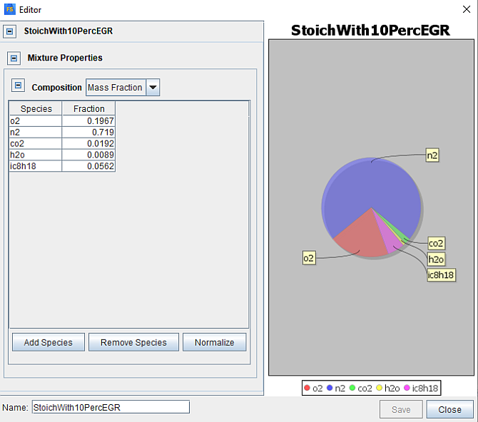
o2=0.1967
h2o=0.0089
co2=0.0192
ic8h18=0.0562
n2=0.7190
To do this, select Create new gas mixture... in the
Composition drop-down list above the Location list and click the
Pencil ![]() icon. This opens the Gas Mixture panel, where you select Add
Species and then choose the species you want from the mechanism (see Figure 5.2: Gas Mixture Editor: Defining Inlet gas composition
). You can find a species more quickly by typing
(the beginning of) the species name to filter the list. Save the inlet gas mixture as
StoichWith10PercEGR. Define turbulence using Turbulent Kinetic Energy and Length
Scale with values of of 7,900 cm2
/sec2 and 0.5 cm, respectively.
icon. This opens the Gas Mixture panel, where you select Add
Species and then choose the species you want from the mechanism (see Figure 5.2: Gas Mixture Editor: Defining Inlet gas composition
). You can find a species more quickly by typing
(the beginning of) the species name to filter the list. Save the inlet gas mixture as
StoichWith10PercEGR. Define turbulence using Turbulent Kinetic Energy and Length
Scale with values of of 7,900 cm2
/sec2 and 0.5 cm, respectively.
Outlet: From the Boundary Conditions node, click
the New Outlet  icon and name it Outlet. Select
Pressure_Out from the Location list and select Total
Pressure as the Outlet option. Give the outlet a
Pressure of 0.9 bar, which arises from the
back-pressure of the exhaust system with an Offset Distance to Apply
Pressure of 0.1 cm. Set the Turbulence Boundary Conditions to
Turbulent Kinetic Energy and Length Scale with values of 7,900
cm2/sec2 and 0.5
cm,respectively.
icon and name it Outlet. Select
Pressure_Out from the Location list and select Total
Pressure as the Outlet option. Give the outlet a
Pressure of 0.9 bar, which arises from the
back-pressure of the exhaust system with an Offset Distance to Apply
Pressure of 0.1 cm. Set the Turbulence Boundary Conditions to
Turbulent Kinetic Energy and Length Scale with values of 7,900
cm2/sec2 and 0.5
cm,respectively.
Piston: From the Boundary Conditions node, click
the New Wall  icon and name it Piston. Select the
Piston item in the Location list. Set the Thermal Boundary
Condition to Wall Temperature, Constant with a value of
420 K. Turn ON the Wall Motion
option and set the piston Motion Type to use a Slider
Crank model with a Stroke of 7.95 cm and a
Connecting Rod Length of 13.81 cm with 0.0
Piston Offset. Change the Movement Type to Moving
Surface and accept the default Global Origin Reference
Frame.
icon and name it Piston. Select the
Piston item in the Location list. Set the Thermal Boundary
Condition to Wall Temperature, Constant with a value of
420 K. Turn ON the Wall Motion
option and set the piston Motion Type to use a Slider
Crank model with a Stroke of 7.95 cm and a
Connecting Rod Length of 13.81 cm with 0.0
Piston Offset. Change the Movement Type to Moving
Surface and accept the default Global Origin Reference
Frame.
Intake: Click the New Wall icon and name it Intake. Select the
IntakeManifold item in the Location list and set the Wall
Temperature to 300 K.
Exhaust: Click the New Wall icon and name it Exhaust. Select the
ExhaustManifold item in the Location list and set the Wall
Temperature to 650 K.
Liner: Click the New Wall icon and name it Liner. Select the
Liner item in the Location list and set the Wall
Temperature to 385 K.
Head: Click the New Wall icon and name it Head. Select the
Head item in the Location list and set the Wall
Temperature to 385 K.
Intake Valves: Click the New
Wall icon and name it IntakeValve1. The valve specification
is a little more complicated than the stationary walls, therefore several steps are required
within the wall panel. These steps specify the wall motion and the way we want the mesh to adapt
to the gap opening near the valve seat when the valve opens or closes.
Select both the IntakeValve1_Seat and IntakeValve1_Stem items in the Location list.
Check the Heat Transfer option and set the Wall Temperature to the constant value of 385 K.
Turn ON (check) the Wall Motion and set the Motion Type to Offset Table.
Accept the default Global Origin for the Reference Frame. Select Spherical for the Coord. System under Direction for the valve motion and set
 =199 degrees and
 =0.0 degrees.
 To import the lift profile (named IntakeLift.csv in the same location as the .stl file you started this tutorial with), select Create New from the Lift Profile drop-down list and click the Pencil
 icon. In the Profile Editor, click the Load CSV
button and navigate to the IntakeLift.csv file.
Accept the defaults in the import dialog and click OK. At the bottom of
the Profile Editor window, name this IntakeValves. Ensure that the units
in the first column are set to Degrees and the second column is set to
cm. Save the Profile.
icon. In the Profile Editor, click the Load CSV
button and navigate to the IntakeLift.csv file.
Accept the defaults in the import dialog and click OK. At the bottom of
the Profile Editor window, name this IntakeValves. Ensure that the units
in the first column are set to Degrees and the second column is set to
cm. Save the Profile. For Movement Type, change the drop-down menu to Valve. Then select just the surface boundary portion of the valve that comes into contact with the valve seat on the port, as well as the surface boundary that contains the seat region. In this case, select both the IntakeManifold and the IntakeValve1_Seat.
Finally, set the Valve Motion Activation Threshold to 0.1 cm. This indicates that the valve will not open until the lift value specified in the valve-lift profile exceeds this threshold. A smaller value will cause the valves to open sooner, but the mesh refinement required to resolve the gap will be higher. This is a trade-off that will need to be determined based on the goals and outcomes desired from the simulation. In addition to the activation threshold, you may also change the minimum number of cells desired at the smallest gap opening. In this case, accept the default value for Approx. Cells in Gap at Min. Lift of 2.0. Click Apply.
Note: According to Forte best practices, the Valve Motion Activation Threshold should be set to a value between 0.02 cm and 0.05 cm (0.05 cm is a good value to start with). The larger threshold value (0.1 cm) is used in this tutorial because the quality of the surface geometry is poor, the valves cannot be tightly seated in the surface mesh, and using a value smaller than 0.1 cm in this specific case may lead to meshing difficulty. Follow the best practices when you set up a new project for production runs. See Forte Best Practices for guidance.
Follow the same procedure to set the boundary conditions for IntakeValve2. This time you can copy and paste the existing IntakeValves profile instead of creating a new one. And for IntakeValve2, the Location selected should be IntakeValve2_Seat and IntakeValve2_Stem, while the surfaces selected under Multiselect the Valve Seat and Surface it Contacts should be the IntakeManifold and IntakeValve2_Seat.
Exhaust Valves: Click the New
Wall icon and name it ExhaustValve1. Follow a similar
procedure as for the Intake Valves. This time, select the
ExhaustValve1_Seat and ExhaustValve1_Stem items in the
Location list and set the Wall Temperature to 497 K.
Turn ON the Wall Motion and set the Motion Type to
Offset Table. Select Global Origin for the
Reference Frame. Select Spherical for the
Coord. System under Direction and set = -199 degrees and = 0.0 degrees (note that this is the opposite
direction from the intake valves, relative to the z-axis). Similarly to the intake valves, first
import the .csv (named
ExhaustLift.csv ) file, accept the defaults, and name it
ExhaustValves. Then follow the same procedures for specifying the
Movement Type to Valve, selecting the Valve
Seat and Surface it Contacts(ExhaustManifold and
ExhaustValve1_Seat), setting the Valve Motion Activation
Threshold to 0.1 cm and setting Approx. Cells in Gap
at Min. Lift to
2.0..
Follow the same procedure to set the boundary conditions for ExhaustValve2. Use the ExhaustValves profile again for ExhaustValve2, but select the appropriate surfaces for the ExhaustValve2 in the Location list and in the Multiselect the Valve Seat and the Surface it Contacts list.
The domain is initialized with the operating conditions, species concentrations and temperatures. The Default Initialization species composition is at the expected exhaust composition, assuming complete combustion. The intake and exhaust must also be initialized to the boundary condition values. Set the following initialization parameters:
Select Initial Condition > Default Initialization in the Workflow tree. Set the Initialization Order to 2. Since flow goes generally from the intake to the cylinder and then to the exhaust, this indicates that this default (cylinder) region will be the second in the initialization order precedence list.
Select Create new gas mixture... in the Composition drop-down list and click the Pencil
icon. This opens the Gas Mixture panel, where you select Add
Species, set to a Mass Fraction of n2=0.7192,
co2=0.1923 and h2o=0.0885 and Save this
composition as ExhaustEst_w10percEGR.Set a Temperature of 1,000 K and the Pressure to 1.0 bar.
For Turbulence initialization, use the Turbulent Kinetic Energy and Length Scale option with values of 7,900 cm2/sec2 and 0.4 cm, respectively.
The Velocity is initialized using Engine Swirl, with an Initial Swirl Ratio of -0.0739, an Initial Swirl Profile Factor of 3.11, and checking (ON) Initialize Velocity Components Normal to Piston.
Click Apply.
Intake Initialization: The intake manifold Initial Condition is set to match the Boundary Condition at the Inlet. Since this is a separate port that can be closed off from the main cylinder region, we also need to set the equivalent of a material point to identify the region, as well as an initialization order that helps determine what region takes precedence in initializing new cells that appear when gaps are opened.
From the Initial Conditions Workflow tree item, select the New Secondary Region From Material Point
 icon and name it Intake.
To identify the region, select a point for the Location under the Reference Frame selection, which is a point that will always be within the Intake port. Set the coordinates for this case to X=6.0, Y=2.0, Z=5.0 cm, which is a point just inside the inlet.
Set the Initialization Order to 1. Flow is expected to go from the intake to the main region; for this reason, we give it the first order in initialization precedence.
Set the Composition by selecting in the previously saved profile, StoichWith10PercEGR. Set the Temperature to 300 K and Pressure to 0.8 bar.
For Turbulence initialization, use the Turbulent Kinetic Energy and Length Scale option with values of to 7,900 cm2/sec2 and 0.5 cm, respectively. Click Apply.
Exhaust Initialization: The Initial Conditions of the Exhaust is set to match the Boundary Condition of the Outlet.
From the Initial Conditions Workflow tree item, select the New Secondary Region From Material Point icon
and name it Exhaust. To identify the region, select a point for the Location under the Reference Frame selection, which is a point that will always be within the ExhaustPort region. Set the coordinates for this case to X= -4.0, Y=2.0, Z=2.0 cm, which is a point just inside the outlet.
Set the Initialization Order to 3. Flow is expected to go from the cylinder to the exhaust port; for this reason, we give it the last order in initialization precedence for the 3 regions defined.
Set the Composition to the existing profile, ExhaustEst_w10percEGR. Set the Temperature to 650K and Pressure to 0.9 bar.
For Turbulence initialization, use the Turbulent Kinetic Energy and Length Scale option, with values of 7,900 cm2/sec2 and 0.5cm, respectively. Click Apply.
Simulation controls allow you to define the simulation limits, time step, chemistry solver and transport terms.
Simulation Limits: Use the Simulation Controls panel to select a Crank Angle Based simulation from a crank angle of 340 to 900 degrees. Set RPM = 1,500 rpm. The engine Cycle Type is 4-Stroke. Click Apply.
Time Step: Use Simulation Controls > Time Step and set the following parameters:
Initial Simulation Time Step to 5.0E-7 seconds
Enable Restrict Time Step by Crank Angle
Max. Crank Angle Delta Per Time Step of 1.1 degrees
Set the Max. Time Step Option to Constant and set the value of Max. Simulation Time Step to 3.E-5 sec. The time step will be adaptively determined throughout the simulation, based on local solution gradients, so this just sets the maximum value allowed. In this tutorial case, a relatively large constant max dt (3.E-5 sec) is used to reduce the simulation time. In production runs, Forte best practices recommend that the max dt be controlled so it is no larger than 5.E-6 sec when flame propagation or spray is active, which can be achieved by using a time-varying max dt profile.
The Advanced Time Step Control Options settings are kept at the defaults. Click Apply.
Time Step Growth Factor = 1.3
Fluid Acceleration Factor = 0.5
Rate of Strain Factor = 0.6
Convection factor = 0.2
Internal Energy Factor = 1.0
Max. Convection Subcycles = 8
Chemistry Solver: Simulation Controls > Chemistry Solver is also kept at the defaults, with the following parameters:
Absolute Tolerance = 1.0E-12
Relative Tolerance = 1.0E-5
Use Dynamic Cell Clustering to take advantage of groups of cells with similar conditions. Select 2 features to introduce Dynamic Cell Clustering: 1) Max. Temperature Dispersion of 10 K and 2) a Max. Equilibrium Ratio Dispersion of 0.05.
To increase the time-to-solution speed, you have the ability to choose when chemistry is activated. In this tutorial, select Activate Chemistry Conditionally, and select When Temperature is Reached with Threshold Temperature 600 K and also select During Crank Angle Interval with crank angles between 650 and 850 degrees. This ensures that chemistry is active during the time that combustion is expected even if temperature does not rise above 600 K. Click Apply.
Transport Terms: Use the default transport tolerances and maximum number of iterations.
Output controls determine what data are stored for viewing during the simulation and for creating plots, graphs and animations in Ansys EnSight.
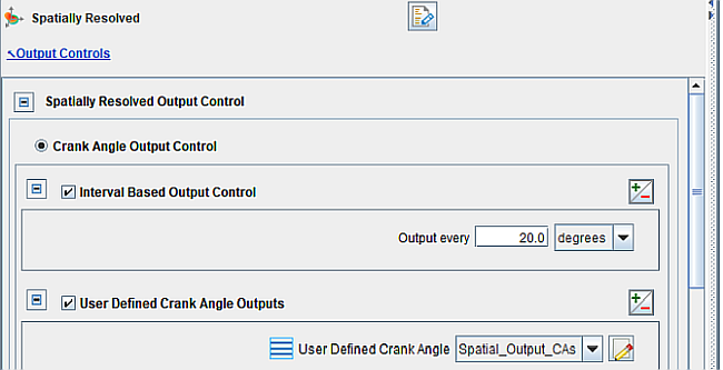
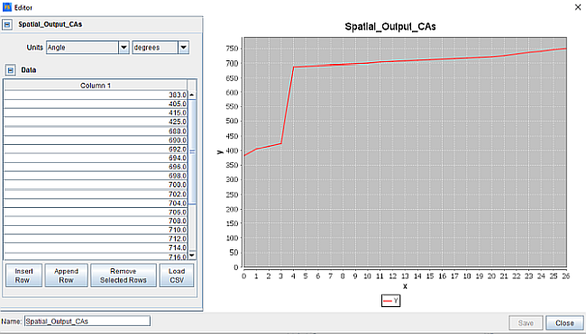
Spatially Resolved: Allows you to control when spatially resolved data such as velocity, temperature, species concentrations, etc., will be output. In the Spatially Resolved panel, set the Output Timing Control to Crank Angle, and turn ON (check) Interval Based Crank Angle Outputs, set to report every 20 degrees (to manage the size of the output file). You can optionally increase the frequency of output during the cycle by selecting User Defined Output Control and importing the Spatial_Output_CAs.csv file, which has a list of specific crank angles where spatially resolved output will occur (illustrated in Figure 5.3: Output control panel - Spatially Resolved ). Alternatively, you could select User Defined Output Control, and use the Profile Editor to create some other file specifying an output crank-angle profile (the provided profile is illustrated in Figure 5.4: User-defined spatially resolved output controls ). Select the following species for Spatially Resolved Species: h2o, no, no2, co, co2, o2, ic8h18 and n2.
Spatially Averaged And Spray: Allows you to control the output of values that are averaged across the domain. In the Spatially Averaged panel, set the Crank Angle Output Control to reporting every 1 degree. Select the following species for Spatially Averaged Output: h2o, no, no2, co, co2, o2, ic8h18, and n2. Click Apply.
Restart Data: If you anticipate that the case will be stopped and you want the ability to restart it from the last time step solved, select Output Controls > Restart Data. You can specify certain Restart Points using a separate file. Turn ON (check) User Defined Restart Points and use the Profile Editor to create a Restart profile. You can view, edit or import new Restart Points in this 1-D Profile Editor. Sometimes it is helpful in spark ignition cases to save a restart file after IVC but before the spark occurs (CA=687 in this case) so you can use the compression portion of the cycle as a start point in additional runs. Create a new profile for this purpose called RestartOutput and add one line with CA value set to 680. Click Apply.
As a method for checking the automatically generated mesh, you can generate a Preview Mesh.
Select Preview Simulation > Mesh Generation. Select Crank
Angle as the Time Option and set
Start to 720.0 degrees. Enter the
Data Set Name as FTDC. Check the Include
Volume Mesh option and then click the Generate Mesh  icon. Then select the Data Set Name to view in
EnSight. If you want to see the cut plane where the mesh will be generated, create a clip plane
in EnSight. Select all parts and then select Create > Clips.... Use
XYZ as Tool and Mesh Slice Y with Value =
0.0, and then click Create with selected parts. It is a good
practice to look at meshes at key points in the cycle such as Firing Top Dead Center (FTDC),
Exhaust Valve Opening (EVO), Intake Valve Closed (IVC), Intake Valve Open (IVO) and Exhaust Valve
Closed (EVC). You can create a preview mesh similarly by using the following information:
icon. Then select the Data Set Name to view in
EnSight. If you want to see the cut plane where the mesh will be generated, create a clip plane
in EnSight. Select all parts and then select Create > Clips.... Use
XYZ as Tool and Mesh Slice Y with Value =
0.0, and then click Create with selected parts. It is a good
practice to look at meshes at key points in the cycle such as Firing Top Dead Center (FTDC),
Exhaust Valve Opening (EVO), Intake Valve Closed (IVC), Intake Valve Open (IVO) and Exhaust Valve
Closed (EVC). You can create a preview mesh similarly by using the following information:
FTDC @ CA=720: Mesh Slice Y (Value=0.0 cm)
EVO @ CA=192: Mesh Slice Y (Value=2.0 cm)
IVC @ CA=601: Mesh Slice Y (Value=2.0 cm)
IVO @ CA=363: Mesh Slice Y (Value= –1.0 cm)
The settings here depend on the system and environment for your simulations. The default for the Run Settings panel is to have nothing selected.
Run Options: For this tutorial, ensure the check boxes here are unchecked (OFF). You may choose to adjust other settings as necessary for your environment.
Windows Settings: This tutorial does not require changes to this panel's defaults; adjust them as necessary for your environment.
Linux Settings: This tutorial does not require changes to this panel's defaults; adjust them as necessary for your environment.
To complete the lesson, select the Nominal run under Run Simulation on
the Workflow tree and click the blue arrow Start button. You can monitor the
results by clicking on the Monitor Runs  icon. In the Monitor window that opens, you can select the run you wish to
monitor.
icon. In the Monitor window that opens, you can select the run you wish to
monitor.
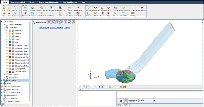
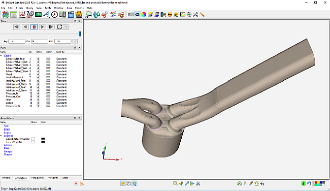
To view the results of the simulation, open Ansys EnSight. In EnSight, open the solution file for the case ( Nominal.ftres ). Figure 5.5: Screen view of the solution file in EnSight shows the screen view once the solution file has been loaded.
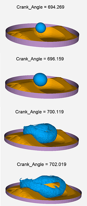
We are interested in creating some average line plots for Pressure, Apparent Heat Release Rate (Apparent HRR) and emissions such as CO and NOx vs. Crank Angle. The thermo.csv file is used to create line plots for Pressure, Apparent HRR, NO, and CO. These figures are shown as Figure 5.6: Pressure and Apparent heat release rate vs. crank angle and Figure 5.7: NO and CO emissions g/kg-fuel) vs. crank angle. Another interesting feature is to use the Iso-Contour Wizard to track the flame front across the cylinder volume using the iso-contour wizard in EnSight, as shown in Figure 5.8: Iso-contours at 1000 K showing the progression of the flame front from CA 694-702 degrees. Use a temperature value of 1000 K for this purpose.
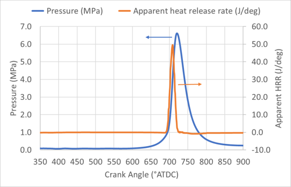
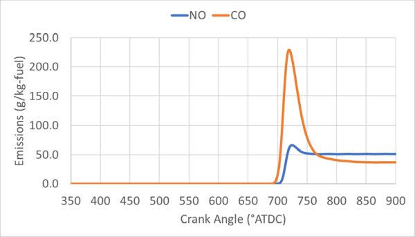
Figure 5.8: Iso-contours at 1000 K showing the progression of the flame front from CA 694-702 degrees