37.5. Mesh Adaption inside Fluent Aero

This tutorial illustrates how to conduct a mesh adaption simulation within Fluent Aero to improve the precision of numerical results and how to post-process these results at each mesh adaption cycle. Inside Fluent Aero, you can now enable mesh adaption for all conditions, design points, defined in a simulation. The current mesh adaption inside Fluent Aero uses by default the polyhedral unstructured mesh adaption called PUMA in conjunction with the Combined Hessian Indicator of Fluent. Mesh adaption cycles are used to progressively refine the baseline mesh to reveal the most salient flow features such as shocks, wakes, etc. Inside Fluent Aero, the baseline mesh, the mesh of your imported case or mesh file, will be automatically reloaded between design points. This guarantees that, at each design point, mesh adaption starts from the coarsest mesh of your simulation, the baseline mesh.

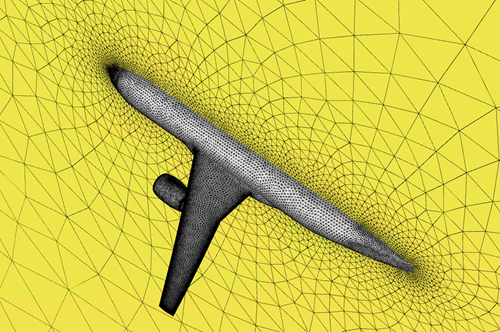
In this tutorial, an aircraft, the NASA Common Research Model (CRM) with a wing-body-nacelle pylon (WBNP) configuration, is employed to illustrate this feature. The flight conditions used in this tutorial correspond to the climb and nominal cruise conditions described in Introduction to Aircraft Component Groups and Computing Aerodynamic Coefficients on an Aircraft at Different Flight Altitudes and Engine Regimes, and are for demonstration purposes only (Completing the previous tutorial is not required). Only four mesh adaption cycles are conducted to demonstrate the capabilities of the tool without necessarily achieving a mesh independent solution.

Note: The main workflow to set-up a mesh adaption simulation in Fluent Aero is described below:

Set up a simulation with one or multiple design points (conditions).
Enable beta features.
File → Preferences... → Aero → Beta Features
Enable Mesh Adaption.
Setup → Advanced Workflows → Adaption
An Adaption node will automatically be displayed under Solution.
Go to Solution → Adaption to set up the mesh adaption settings.
Go to Solution → Files → Intermediate DP Case & Solution Files → Write Per Cycle to save adapted solutions at end of each mesh adaption cycle if needed.
Go to Solution → Solve → Number of Cycles and Iterations to set the total number of cycles and number of iterations per cycle for each design point.
Go to Solution → Solve → Iterations to set the total number of iterations per cycle for each design point.
In the Input:Design Points table to the right, set the design point Status to Needs Update.
Click Solution → Solve Update to launch the airflow simulation with mesh adaption.

The current limitation of the mesh adaptation beta feature in Fluent Aero is as follows:

Saving or reloading mesh adaptation settings for each design point is not supported.

As the adapted mesh size increases with mesh adaption cycles, the computational resource requirements increase. In order to conduct this tutorial, you should have at least 40 GB of disk space and to run using 16 CPUs with 96 GB of RAM.

Download the fluent_aero_tutorial.zip file here .

Unzip fluent_aero_tutorial.zip to your working directory.

Extract the CRM_WBNP_Aircraft.msh.h5 file for this tutorial. The grid consists of 1.2M nodes and 2.4M cells. Five layers of prisms are grown off the aircraft’s wall boundaries and the remainder of the computational domain is filled with tetrahedral cells. The limits of the computational domain are defined by a hemispherical boundary defined as a pressure-farfield boundary type, and a flat circular boundary defined as a symmetry plane in the Z direction. This .msh file therefore meets requirements stated under General Case File or Mesh File Requirements. However, the mesh is very coarse and should be used for demonstration purposes only.

Figure 37.29: View of the Mesh Around the Aircraft

Launch Fluent on your computer. In the Fluent Launcher panel, set the Capacity Level to Enterprise. Then select Aero. Set the number of Solver Processes to 16 or more if possible. Click Start.
In the Fluent Aero workspace, go to File → Preferences.... In the Preferences window, go to the Aero menu and ensure Use Custom Solver Launch Settings, Show Solution Workspace and Enable Solution Workspace Graphics are disabled. Disabling these settings is the preferred approach for running Fluent Aero simulations on your local machine. Inside this window, enable Beta Features to access the mesh adaption capabilities in Fluent Aero.
Follow Step 3 to Step 18 in Introduction to Aircraft Component Groups and Computing Aerodynamic Coefficients on an Aircraft at Different Flight Altitudes and Engine Regimes to create a new project and set up the simulation using two design points. Name the simulation CRM_WBNP_Aircraft_adapt instead of CRM_WBNP_Aircraft in Step 4:
Note: If you have already completed tutorial Introduction to Aircraft Component Groups and Computing Aerodynamic Coefficients on an Aircraft at Different Flight Altitudes and Engine Regimes, you can duplicate its simulation to quickly create an adaption simulation in Fluent Aero. To do so, follow these steps:
1. Double-click to open your Fluent_Aero_Tutorial_03 project under Project Library.
2. Right-click on the CRM_WBNP_Aircraft main tree node in the Project View and then select Duplicate. This simulation contains information that will be reused for this tutorial (mesh, convergence settings, etc.).
3. A New Simulation popup window appears. Enter CRM_WBNP_Aircraft_adapt under Name of the New Simulation. Click OK to close the window. A new simulation called CRM_WBNP_Aircraft_adapt will be automatically loaded in Fluent Aero.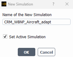
In the Input: Design Points table, edit the Mach Number and Angle of Attack [deg] columns for DP-2 to 0.95 and 3.0 degrees, respectively.Set the Status column of both design points to Needs Update.
Note: The flight condition of DP-2 was modified to clearly observe the benefits of mesh adaption to capture shocks.
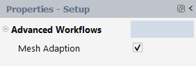
Click Outline View → Setup. In the Setup panel, enable Mesh Adaption under Advanced Workflows to reveal the Adaption node under the Solution.
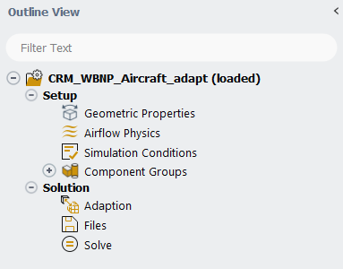
Note: Fluent Aero conducts mesh adaption cycles per design point using PUMA with the Combined Hessian Indicator. At each design point, a baseline mesh solution is used to start the first adaption cycle.
Click on Solution → Adaption to set up mesh properties to preserve or respect at the start of each mesh adaptation cycle. A cycle includes a mesh adaptation step based on the previous solution and mesh, followed by several CFD solver iterations on the adapted mesh.
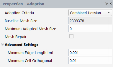
In the Properties – Adaption window,
- Set the Maximum Adapted Mesh Size to 0.
- Set the Minimum Edge Length [m] to 0.001.
- Set the Minimum Cell Orthogonal to 0.01.
  Note: The Properties – Adaption window contains the following mesh adaption settings for PUMA.
  Adaption Criteria:
  The Combined Hessian Indicator is the default Error-based mesh adaption criteria of Fluent Aero. Other Hessian indicators are supported by selecting Case settings. These indicators should be defined inside the imported case file or via the Solution Workspace that is connected to Fluent Aero.
  Baseline Mesh Size:
  This is the mesh cell count of the baseline mesh. This mesh is the grid inside the imported case or mesh file used to create the simulation folder. The baseline mesh is automatically reloaded at the beginning of each design point.
  Maximum Adapted Mesh Size
  This is the maximum number of cells that mesh adaption can produce. It sets an approximate limit to the total cell count of the mesh. The default value is zero and indicates that there is no mesh size constraint during mesh adaption.
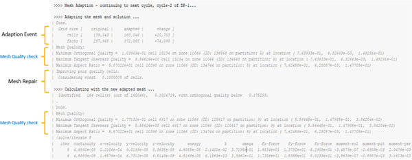
  Mesh Repair
  This option allows you to improve the mesh quality by conducting mesh smoothing after the creation of an adapted mesh within a cycle. In this case, 0.1% of the cells that exhibit the lowest orthogonal quality are repaired. For more information on this option, consult Improving the Mesh by Smoothing and Swapping. When this option is enabled, the following extra steps are automatically added right after the creation of an adapted mesh:
  Mesh Quality Check
  Mesh Repair
  Mesh Quality Check
  Below is an example of the steps that will be printed to the Console when the Mesh Repair option is enabled.
  Minimum Edge Length [m]
  This is the minimum edge length of a cell to respect. A value of zero imposes no restriction.
  Minimum Cell Orthogonal
  This is the minimum cell orthogonal quality that the code aims to maintain in cells resulting from adaptation. Poorer quality cells will have values closer to 0, while higher quality cells will have values closer to 1. This option is unavailable for 2.5D cases.
Go to Solution → Files to set up file write options.
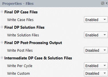
In the Properties – Files window,
- Set Write Case Files to Enabled.
- Set Write Solution Files to Enabled.
- Set Write Post Files to Disabled.
- Set Write Per Cycle to Enabled.
- Set Write Custom to Disabled.
Note: Writing intermediate solutions allows you to inspect the adapted solutions at end of each mesh adaption cycle. The files are named as out.000x.cycle.0x.cas/dat.h5. If Write Per Cycle is Disabled, only the final adapted solution is saved and only this solution can be post-processed.
Go to Solution → Solve.
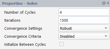
- Set the Number of Cycles to 4, and Iterations to 1500.
  In this case, Number of Cycles represents the total number of cycles conducted for a given design point and not an increment in number of cycles and Iterations represents the maximum number of iterations to perform per mesh adaption cycle for each design point.
- Keep Convergence Settings to Robust to improve convergence as the mesh gets adapted.
- Set Convergence Criteria to Disabled to run 6,000 iterations for each design point.
  Note: Number of Cycles will only be displayed when Mesh Adaption is selected under Advanced Workflows. Initialize Between Cycles allows you to re-initialize the airflow domain at the beginning of each cycle. Details of airflow initialization settings can be accessed under Solve → Convergence Settings → Custom → Initialization.
Click the Update button at the bottom of the Properties - Solve panel to launch the mesh adaption calculations.
When conducting mesh adaption simulations in Fluent Aero, the baseline mesh file of the simulation is created from the imported case file. This mesh is then saved inside -baseline.cas.h5 file and is located in the simulation folder. Fluent Aero will automatically reload the baseline mesh file at the beginning of each design point.
During a mesh adaption simulation, the first adaption cycle consists in running an airflow solution on the baseline mesh. Then, at the beginning of the 2^nd cycle, mesh adaption is carried out on the 1^st cycle mesh using its solution. Mesh cells within the domain will be refined or coarsen based on the adaption’s predefined criteria. A new mesh is therefore generated and the previous solution is interpolated onto that mesh. Calculations will resume and continue until they reach their assigned number of iterations per cycle since Convergence Criteria has been set to Disabled. This procedure is repeated until all adaption cycles have been ran. Since solutions are interpolated between adaption cycles, large fluctuations can be observed in the plots of residual, lift/drag, and mesh cell count at the beginning of each cycle.
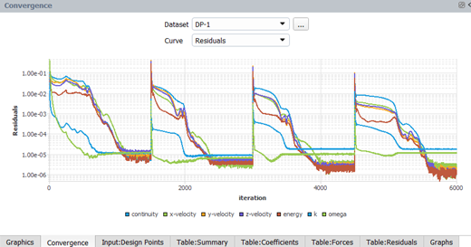
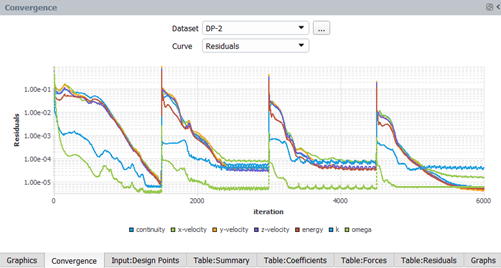
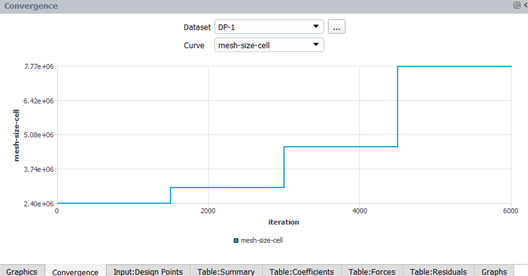
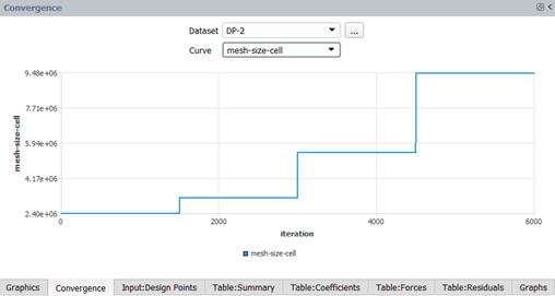
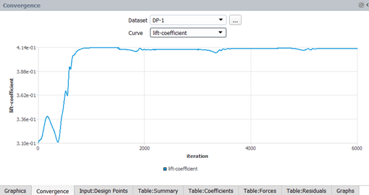
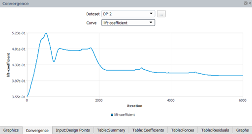
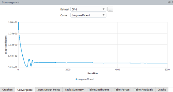
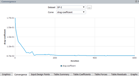
You can monitor the adaption simulation of each design point in the Convergence window on the right of your screen. The start of each adaption cycle can be easily observed by the jumps in Residual, lift-coefficient, and drag-coefficient plots. In addition, a mesh-size-cell curve can be used to monitor the size of the adapted meshes produced at each mesh adaption cycle. In this tutorial, the mesh adaption events can be seen at iteration 1500, 3000, and 4500 in Figure 37.30: Residuals of DP-1 and DP-2, Figure 37.31: Mesh-size-cell of DP-1 and DP-2, Figure 37.32: Lift Coefficient of DP-1 and DP-2 and Figure 37.33: Drag Coefficient of DP-1 and DP-2.
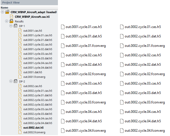
Once your simulations are complete, both case and data files are saved at the end of each mesh adaption cycle and are located in the Project View, under both DP-1 and DP-2 folders. Moreover, all files are physically written to the Results folder of your simulation project. To do see where they are written, right-click on the Results folder in the Project View. Select Open in File Explorer to view these files and all contents of Results. The out.000x.cas/dat.h5 files contain the final adapted solutions of each design point while the out.000x.cycle.0x.cas/dat.h5 are the adapted solutions at end of each mesh adaption cycle of a given design point.
Note: Cycling workflows involves the calculation of multiple simulation cycles within a given design point. In this case, the airflow simulation and its total number of iterations are subdivided into a given number of cycles and number of iterations per cycle. There are two types of cycling workflows in Fluent Aero:
- Solution → Advanced Workflows → Parameter Search
- Solution → Advanced Workflows → Mesh Adaption
In the Input: Design Points table, a design point simulation with cycles can be assigned a different Status:
- Needs Update
- Continue To Update
- Restart from Restart Cycle
These options apply to all cycling workflows in Fluent Aero.
- Needs Update
  Begins from the baseline mesh and runs with the total number of cycles defined in the Properties – Solve panel.
- Continue To Update
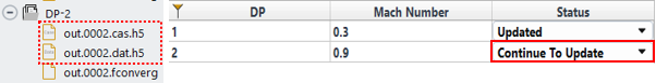
  Uses the final solution to continue a simulation with or without cycles. This option can be applied in four scenarios, described below, using a design point with five or ten mesh adaptation cycles as examples:
  Mesh Adaption disabled → Continue To Update → Mesh Adaption disabled.
  Standard usage of the Continue To Update option.
  Mesh Adaption disabled → Continue To Update → Mesh Adaption enabled (five cycles)
  In this case, Continue To Update allows you to carry out 5 cycles using the solution with Mesh Adaption disabled. The first cycle runs the baseline solution, and mesh adaption begins at the start of the second cycle. This is similar to running mesh adaption from scratch. The total cycle count will be five.
  Mesh Adaption enabled (5 cycles) → Continue To Update → Mesh Adaption disabled.
  Here, Continue To Update lets you add more iterations to the final adapted solution. Specify additional iterations to continue simulating the last adapted cycle (in this case, the fifth). No new cycles will be added. Note that the results of the extra iterations are saved to final output files, not the existing cycle 5 solution files.
  Mesh Adaption enabled (5 cycles) → Continue To Update → Mesh Adaption enabled (10 cycles).
  In this case, Continue To Update allows you to add five more cycles to an existing simulation with five mesh adaption cycles. The final solution from the initial five cycles is used to continue the simulation. Set Number of Cycles to 10 (the total cycle count) rather than five. You can also adjust the number of iterations per cycle if desired.
- Restart from Restart Cycle
  Restarts the simulation from a specified cycle until the maximum Number of Cycles set in Properties – Solve is reached. To restart from a given cycle, the case and data files for that specific cycle must have been saved in the previous mesh adaptation or parametric search simulation, as these files are needed to restart the simulation. To specify the cycle to restart or recompute, an extra Restart Cycle column will appear in the Input:Design Points table after selecting Restart under the Status column.
  To better illustrate the usage of this restart capability, two scenarios are presented below. In each of these scenarios, five mesh adaption cycles have already been obtained before conducting a restart simulation from the third cycle.
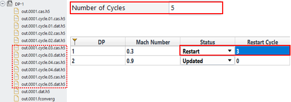
  Mesh Adaption enabled
  In this case, Restart will allow you to restart the mesh adaption from cycle 3 until cycle 5 is completed. If you would like to run for more cycles, you can do so by changing the Number of Cycles in Properties – Solve panel.
  Mesh Adaption disabled
  In this case, Restart will allow you to rerun cycle 3 for the prescribed number of Iterations specified in the Properties – Solve panel. Cycles 4 and 5 solution will be deleted.

Go to the Convergence window. Set Dataset to DP-1 and then DP-2 and observe their Residual, mesh-size-cell, lift-coefficient, and drag-coefficient history by selecting these options next to Curve.

Figure 37.30: Residuals of DP-1 and DP-2

Figure 37.31: Mesh-size-cell of DP-1 and DP-2

Figure 37.32: Lift Coefficient of DP-1 and DP-2

Figure 37.33: Drag Coefficient of DP-1 and DP-2

From the above figures, good residual convergence is maintained thought out the entire mesh adaption process. Moreover, aerodynamic coefficients seem to converge towards a unique solution that is different than the baseline solution, for instance DP-2.

The table below lists the values of lift and drag coefficients at each adaption cycle of DP-1 and DP-2.

Table 37.3: Lift and Drag Coefficients at Each Adaption Cycle of DP-1

DP-1	1500^th iteration	3000^th iteration	4500^th iteration	6000^th iteration
C_L (Lift-Coefficient)	0.414004	0.412024	0.413292	0.413170
∆C_L	–	0.001980	0.001268	0.000122
C_D (Drag-Coefficient)	0.0492498	0.0487949	0.0481736	0.0479268
∆C_D	–	0.0004549	0.0006213	0.0002468

Table 37.4: Lift and Drag Coefficients at Each Adaption Cycle of DP-2

DP-2	1500^th iteration	3000^th iteration	4500^th iteration	6000^th iteration
CL (Lift-Coefficient)	0.476427	0.424353	0.417236	0.410279
∆C_L	–	0.052074	0.007117	0.006957
C_D (Drag-Coefficient)	0.089989	0.0881000	0.0877869	0.0876705
∆C_D	–	0.0018890	0.0003131	0.0001164

The above table confirms the trend observed in the Convergence plots as lift and drag coefficients converge towards a unique solution and their differences (∆C_L and ∆C_D) between adaption cycles decrease.

Go to Outline View → Results → Design Point. Under the Properties - Design Point panel, set Design Point to Load to 2 . Click Load Design Point. This will load the final adapted airflow solution for DP-2.
You can create graphics to quickly post-process the final adapted mesh and airflow solution of DP-2 from the Results node under the Outline View.
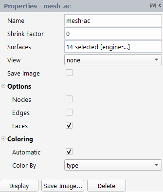
- Click on Meshes under Graphics, then click New in the Properties – Meshes panel to create a new mesh display object named mesh-1. Click on mesh-1 and follow the steps below:
  - Change the Name to mesh-ac.
  - Set Surfaces to Wall type so that all walls of the CRM aircraft are selected.
  - Enable Options → Faces is enabled. Disable Nodes and Edges.
  - Click Display in the Properties panel to show the aircraft in the Graphics window.
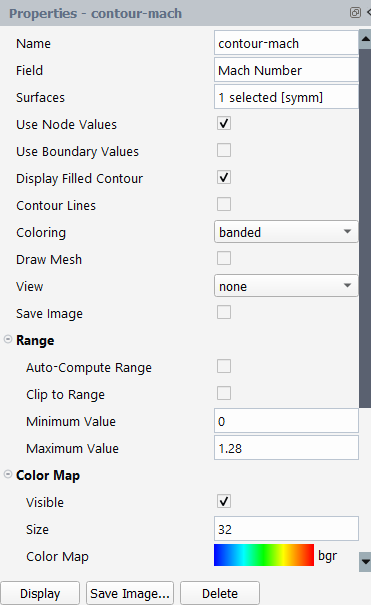
- Right-click on Contours under Graphics and select New to create a new contour-1 object. In the Properties - contour-1 panel, do the following:
  - Change the Name to contour-mach.
  - Set Field to Mach Number.
  - Set Surfaces to Symmetry type to select the symmetry plane.
  - Set Coloring to banded.
  - Disable Auto-Compute Range under Range. Set Minimum Value and Maximum Value to 0 and 1.28, respectively.
  - Under Color Map,
    Set Size to 32.
    Set Color Map to bgr.
  - Click Display in the Properties - mesh-ac panel to show the symmetry plane in the Graphics window.
- Under Results → Design Point, right-click on Scene then select New to create a scene object.
  - Click on the new scene-1 object under Scene.
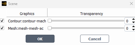
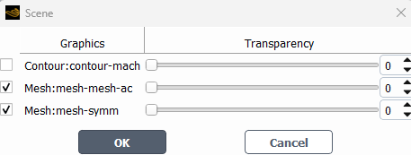
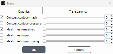
  - In Properties – scene-1 panel, click the text box next to Graphics Objects to bring up the Scene window. Then enable Contour: contour-mach and Mesh:mesh-ac under the Graphics column. Click OK to close the window.
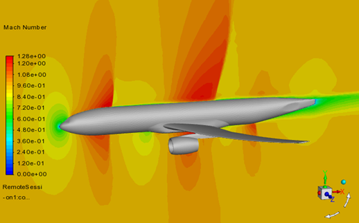
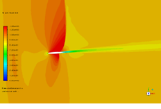
  - Click Display at the bottom of the Properties – scene-1 panel. The output view of scene-1 is displayed in the Graphics window. Zoom in on the aircraft to match the image shown in Figure 37.34: Mach Number on Symmetry Plane of DP-2’s Solution at the Last Adaption Cycle.
  Figure 37.34: Mach Number on Symmetry Plane of DP-2’s Solution at the Last Adaption Cycle
  
  The figure above shows the Mach number field at the symmetry plane of the final adapted airflow solution of design point 2. Since the incoming airflow of design point 2 is close to sonic conditions, Mach 0.95, airflow reaches sonic speed after being accelerated by the aircraft’s geometry. Shocks as well as their locations are precisely captured over the fuselage.
You can also display the final adapted mesh of design point 2 by following these steps:
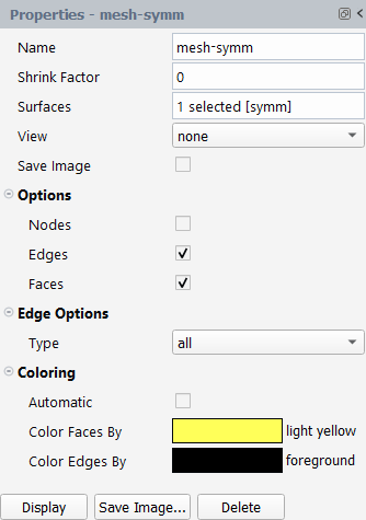
- Click on Meshes under Graphics, then click New in the Properties – Meshes panel to create a new mesh display object named mesh-1. Click on mesh-1 and do the following under its Properties panel:
  - Change the Name to mesh-symm.
  - Set Surfaces to Symmetry type so that the symmetry plane is selected.
  - Enable Options → Edges and Faces. Disable Nodes.
  - Under Coloring, disable Automatic. Set Color Faces By to light yellow and set Color Edges By to foreground.
  - Click Display in the properties panel to update mesh-symm settings.
- Click on the scene-1 object under the Scene node.
  - In Properties – scene-1 panel, click on the text box next to Graphics Objects to bring up the Scene window again. Disable Contour: contour-mach under the Graphics column. Enable Mesh:mesh-ac and Mesh:mesh-symm under the Graphics column. Click OK to close the window.
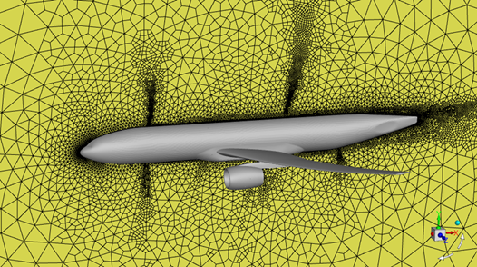
  - Click Display at the bottom of the Properties – scene-1 panel. The output view of scene-1 is displayed in the user interface’s Graphics window shown below.
    Figure 37.35: Adapted Mesh on Symmetry Plane of DP-2’s Solution at the Last Adaption Cycle
    
    The above figure shows the extra mesh refinement, that was added to the baseline mesh by mesh adaption, to capture the most salient features of the solution Figure 37.35: Adapted Mesh on Symmetry Plane of DP-2’s Solution at the Last Adaption Cycle, such as shocks, wakes and the boundary layer over the fuselage.
Right-click onto the mesh-symm object then select Copy to create another mesh object. In the Properties panel of the new mesh object, set its Name as mesh-wing. Click on the Surfaces selection box and ensure that only the walls of the engine and wing are selected. Click Display to view the surface mesh over the wing and engine in the Graphics window as shown in the figure below.
Figure 37.36: Surface Mesh Over the Wing of DP-2 at the Last Adaption Cycle (Adapted Mesh: Top=Left , Bottom=Right)

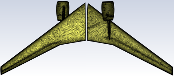
Mesh adaption automatically refines the baseline surface mesh seen in Figure 37.36: Surface Mesh Over the Wing of DP-2 at the Last Adaption Cycle (Adapted Mesh: Top=Left , Bottom=Right) to capture the shock locations over the suction and pressure side of the wing. This allows for a precise representation of the pressure distribution [Figure 37.37: Surface Pressure over the Wing of DP-2’s Solution at the Last Adaption Cycle (Top=left , Bottom=right)] along the wing and consequently of the aerodynamic coefficients.
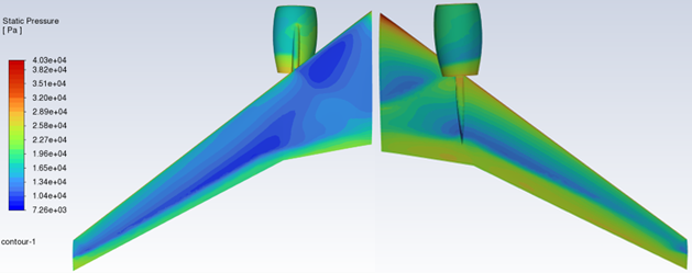
Right-click onto the contour-mach object then select Copy to create another mesh object. In the Properties panel of the new mesh object, set its Name as contour-pressure. Change Field from Mach Number to Static Pressure. Click on the Surfaces selection box and ensure that only walls are selected except for the fuselage walls. Enable Auto-Compute Range under Range. Click Display to view the surface pressure over the wing and engine in the Graphics window as shown in the figure below
Figure 37.37: Surface Pressure over the Wing of DP-2’s Solution at the Last Adaption Cycle (Top=left , Bottom=right)

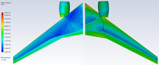
In the above image, the location of the shocks over the wing surface is precisely captured with mesh adaption. The sharp static pressure increase after the shock is better represented by the adapted solution than by the baseline result, Figure 37.37: Surface Pressure over the Wing of DP-2’s Solution at the Last Adaption Cycle (Top=left , Bottom=right). This is mainly due to the extra surface mesh refinement generated by the Combined Hessian Indicator as seen in Figure 37.36: Surface Mesh Over the Wing of DP-2 at the Last Adaption Cycle (Adapted Mesh: Top=Left , Bottom=Right).
Note: You can load the baseline solution to analyze the enhancements provided by mesh adaption to the precision of your CFD calculation. To view the baseline solution, do the following:
1. Go to the Project View and right-click to load the case and data files of the 1st cycle of DP-2, out.0002.cycle.01.cas/dat.h5. The 1st cycle of a mesh adaption simulation in Fluent Aero contains the final CFD solution computed on the baseline mesh.
2. Go to the Outline View and then click Display in the mesh-wing object. The surface mesh before adaption will be displayed as shown in Figure 37.38: Surface Mesh Over the Wing of DP-2 at the First Adaption Cycle (Baseline Mesh: Top=Left , Bottom=Right). Compare this figure to Figure 37.36: Surface Mesh Over the Wing of DP-2 at the Last Adaption Cycle (Adapted Mesh: Top=Left , Bottom=Right) to see that the extra mesh refinement was added to capture the shock at the pressure and suction sides of the aircraft.
3. Go to the Outline View and then click Display in the contour-pressure object. The static pressure over the wing before mesh adaption will be displayed as shown in Figure 37.39: Surface Pressure over the Wing of DP-2’s Solution at the First Adaption Cycle (Top=left , Bottom=right). Compare this figure to Figure 37.37: Surface Pressure over the Wing of DP-2’s Solution at the Last Adaption Cycle (Top=left , Bottom=right) to see the sharp representation of the pressure jump at the shock at the pressure and suction sides of the aircraft.
To load the solution of a different mesh adaption cycle, select its numbered solution file in the Project View and load its corresponding case and data files.
You can then upload the last adaption cycle of DP-2 to continue with the current tutorial. To do this, in the Outline View, go to Results → Design Point and set Design Point to Load to 2.
Figure 37.38: Surface Mesh Over the Wing of DP-2 at the First Adaption Cycle (Baseline Mesh: Top=Left , Bottom=Right)

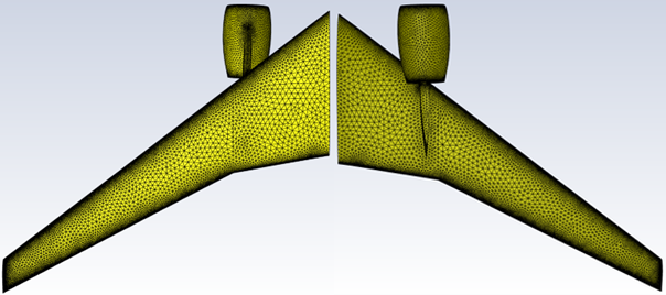
Figure 37.39: Surface Pressure over the Wing of DP-2’s Solution at the First Adaption Cycle (Top=left , Bottom=right)
You may need to examine the results of the airflow calculation within the domain. Go to Results → Design Point (DP-2 Loaded) → Surfaces. Under the Properties – Surfaces panel, click on New → Plane... to create a new cutting plane. Set Creation Mode to XY Plane and Z [m] to 9.7. Go back to Outline View → Surfaces and click on New → Plane... to create an additional cutting plane. This new plane will be named plane-2. Click this plane in the Outline View and set Creation Mode to XY Plane and set Z [m] to 20. The first plane, plane-1, cuts through the engine while the second plane, plane-2, is located near the wing tip.
To display Mach number over cutting plane-1, click on contour-mach under Contours, and set its Surfaces to plane-1. Enable Range → Auto-Compute Range and Use Global Range. Go to Scene→ scene-1 → Graphics Objects and enable both contour-mach and mesh-ac. Click Display.
Repeat the same step to display the Mach number on plane-2. The Mach number contours of plane-1 and plane-2 are shown in the figure below.
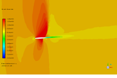
Figure 37.40: Mach Number over the Wing of DP-2’s Solution at the Last Adaption Cycle (Z = 9.7 on the Left and 20 m on the Right)

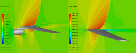
Shocks over the wing and nacelle and at the exhaust are sharply captured by mesh adaption. In addition, the wake produced by the wing and the flow generated by the exhaust are well resolved via mesh adaption.

You can also postprocess the adapted mesh and solutions from each adaption cycle to track how the mesh adaption improves the airflow solution. Fluent Aero can automatically post-process all the cycles of a given design point or of all design points. Follow the steps below to create mesh and Mach number images at z = 9.7 and 20 m of all the mesh adaption cycles of DP-2.

Creating the mesh object (mesh-plane-1)
- Right-click the mesh-symm object and select Copy to create another mesh object. In the Properties panel of the new mesh object, set its Name as mesh-plane-1. Set its Surfaces to Plane-1.
- Adjust the view of the image in the Graphics window to resemble those shown in Table 37.5: Meshes and Airflow Solutions of DP-2 over the Engine at Each Adaption Cycle (Z = 9.7 m). Right-click the mesh-plane-1 object and select Save View. This creates a new view named aero-view-mesh-plane-1. In the Properties panel for mesh-plane-1, select this view under View.
- Enable Save Image in the Properties panel of mesh-plane-1 and click Display.
Creating the contour object (contour-mach-at-plane-1)
- Right-click the contour-mach object, then select Copy to create another contour object. In the Properties panel of the new contour object, set its Name as contour-mach-at-plane-1. Set its Surfaces to Plane-1.
- Adjust the view of the image in the Graphics window to resemble those shown in Table 37.5: Meshes and Airflow Solutions of DP-2 over the Engine at Each Adaption Cycle (Z = 9.7 m). Right-click the contour-mach-at-plane-1 object and select Save View. This creates a new view named aero-view-contour-mach-at-plane-1. In the Properties panel for contour-mach-at-plane-1, select this view under View.
- Enable Save Image in the Properties panel of mesh-plane-1 and click Display.
Repeat both steps above to create an additional mesh object and contour object at cutting plane-2 defined at z = 20 m.
Right-click Results → Design Point (DP-2 Loaded) → Save Current DP Images All Cycles. This will create images of the mesh and Mach contours at plane-1 and plane-2 of DP-2. You will find these images inside the Results directory location. These filenames are shown below.

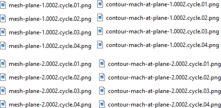
These images can be seen in Table 37.5: Meshes and Airflow Solutions of DP-2 over the Engine at Each Adaption Cycle (Z = 9.7 m) and Table 37.6: Meshes and Airflow Solutions of DP-2 over the Wing at Each Adaption Cycle (Z = 20 m)). They illustrate how the mesh is adapted at each mesh adaption cycle and how the solution improves. Several flow features become more apparent with mesh adaption. For instance:

The shock produced by the exhaust and its interaction with the shear layer that originates from the lip of the nozzle.
The shock produced by the fuselage as it propagates upstream of the nacelle, see Table 37.5: Meshes and Airflow Solutions of DP-2 over the Engine at Each Adaption Cycle (Z = 9.7 m).
The shocks on the pressure and suction sides of the wing are clearly visible as the mesh gets finer. This region receives extra refinement to properly capture the pressure jump across these shocks.
The wakes produced by the wing and nacelle.

Table 37.5: Meshes and Airflow Solutions of DP-2 over the Engine at Each Adaption Cycle (Z = 9.7 m)

	Adapted Mesh	Adapted Solution (Mach Number)
Iteration 1500^th (1^st Cycle with the baseline mesh)		-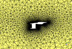
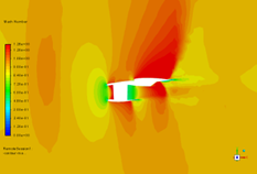
Iteration 3000^th (2^nd Cycle)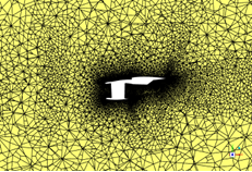
Iteration 4500^th (3^rd Cycle)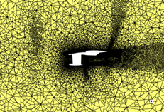
Iteration 6000^th (4^th Cycle)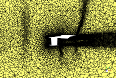

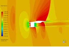
Table 37.6: Meshes and Airflow Solutions of DP-2 over the Wing at Each Adaption Cycle (Z = 20 m))

	Adapted Mesh	Adapted Solution (Mach Number)
Iteration 1500^th (1^st Cycle with the baseline mesh)		-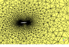
Iteration 3000^th (2^nd Cycle)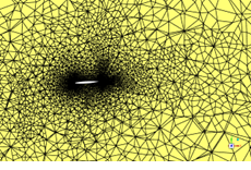
Iteration 4500^th (3^rd Cycle)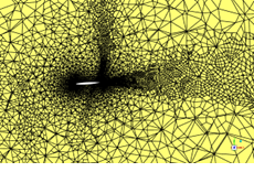
Iteration 6000^th (4^th Cycle)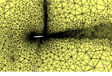

You can also create animations from the figures that were automatically created by Fluent Aero in step 17. This will allow you to clearly see how the solution evolves at each mesh adaption cycle while enhancing its resolution. Follow the steps below to create mesh and Mach number contour animations of DP-2 at z = 7.9 and z = 20.
- Animation of cutting plane meshes at z = 7.9 m
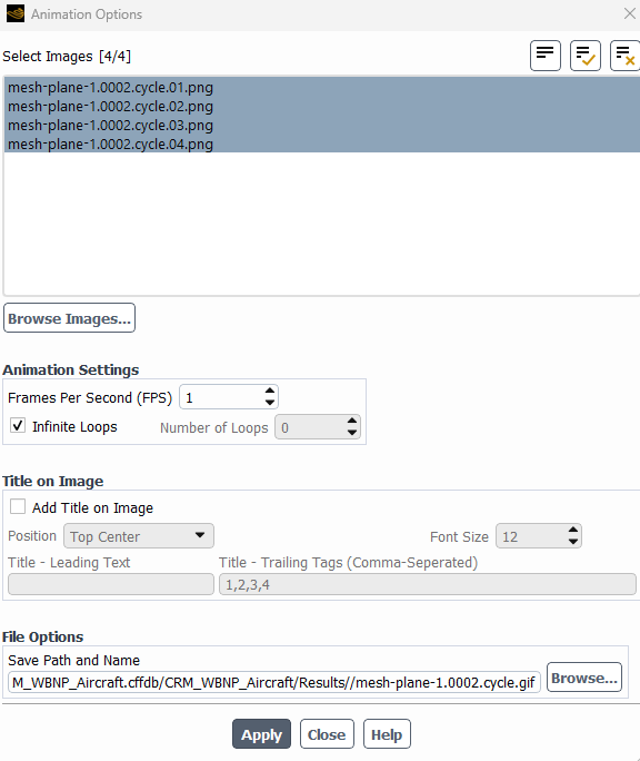
  1. Click on Results → Animation → New Animation from Files... to open the Animation Options window.
  2. Click Browse Images… to navigate to the Results folder.
  3. Hold the Ctrl key to select the image files of mesh-plane-1.0002.cycle.0x.png. Select them in ascending order of cycle.
  4. Set Animation Settings → Frames Per Second (FPS) to 1.
  5. Rename the output file name as mesh-plane-1.0002.gif under File Options → Save Path and Name.
  6. Click Apply to output the animation file.
- Animation of cutting plane Mach number contours at Z = 7.9 m
  Repeat the steps mentioned above to create an animation of Mach number contours using the following images, contour-mach-at-plane-1.0002.cycle.0x.png. Name the output file contour-mach-at-plane-1.0002.gif.
  The following Show-Me animation is presented as an animated GIF in the online help. If you are reading the PDF version of the help and want to see the animated GIF, access this section in the online help. The interface shown may differ slightly from that in your installed product.
  Figure 37.41: DP-2 at Z = 7.9m
- Animations of cutting plane mesh and Mach number contours at z = 20m
  Repeat the steps necessary to create mesh and Mach contour animations at Z = 7.9m in order to create the same animations at Z = 20m. Name them mesh-plane-1.0002.gif and contour-mach-at-plane-2.0002.gif, respectively. The two animations of DP-2 at Z = 20 m are shown as below:
  The following Show-Me animation is presented as an animated GIF in the online help. If you are reading the PDF version of the help and want to see the animated GIF, access this section in the online help. The interface shown may differ slightly from that in your installed product.
  Figure 37.42: DP-2 at Z = 20m
  Note: You can also create animations for DP-1 by following the steps below:
  Select Outline View → Results → Design Point (DP-2 Loaded).
  Set Design Point to Load to 1 under the Properties panel and click Load Design Point.
  Enable Save Image in the Properties panel ofmesh-plane-1 and mesh-plane-2.
  Apply the following settings, under the Properties - contour-mach-at-plane-1 and Properties - contour-mach-at-plane-2.
  Save Image is enabled.
  Range → Minimum Value and Maximum Value are set to 0 and 0.8, respectively.
  Right-click Results → Design Point (DP-1 Loaded) and select Save Current DP Images All Cycles to export images of all objects that have been set to Save Image for DP-1.
  Repeat step 18 to create animations for DP-1.
  The output animations of mesh and Mach number contours of DP-1 at Z = 9.7 and 20 m are shown below. They show how mesh adaption captures the exhaust flow and the wake produced by the wing with great detail.
  The following Show-Me animation is presented as an animated GIF in the online help. If you are reading the PDF version of the help and want to see the animated GIF, access this section in the online help. The interface shown may differ slightly from that in your installed product.
  Figure 37.43: DP-1 at Z = 9.7m
  
  The following Show-Me animation is presented as an animated GIF in the online help. If you are reading the PDF version of the help and want to see the animated GIF, access this section in the online help. The interface shown may differ slightly from that in your installed product.
  Figure 37.44: DP-1 at Z = 20m