3.5. Tutorial - Modeling Flow Through Porous Media

3.5. Tutorial - Modeling Flow Through Porous Media - UTL Edition

3.5.1. Introduction

Many industrial applications such as filters, catalyst beds, and packing, involve modeling the flow through porous media. This tutorial illustrates how to set up and solve a problem involving gas flow through porous media.

The industrial problem solved here involves gas flow through a catalytic converter. Catalytic converters are commonly used to purify emissions from gasoline and diesel engines by converting environmentally hazardous exhaust emissions to acceptable substances. Examples of such emissions include carbon monoxide (CO), nitrogen oxides (NOx), and unburned hydrocarbon fuels. These exhaust gas emissions are forced through a substrate, which is a ceramic structure coated with a metal catalyst such as platinum or palladium.

The nature of the exhaust gas flow is a very important factor in determining the performance of the catalytic converter. Of particular importance is the pressure gradient and velocity distribution through the substrate. Hence, CFD analysis is useful for designing efficient catalytic converters. By modeling the exhaust gas flow, the pressure drop and the uniformity of flow through the substrate can be determined. In this tutorial, Ansys Fluent is used to model the flow of nitrogen gas through a catalytic converter geometry, so that the flow field structure may be analyzed.

This tutorial demonstrates how to do the following in Ansys Fluent:

Use the Watertight Geometry guided workflow to:
- Import a CAD geometry
- Generate a surface mesh
- Cap inlets and outlets
- Extract a fluid region
- Generate a volume mesh
Set up a porous zone for the substrates with appropriate resistances.
Calculate a solution for gas flow through the catalytic converter using the pressure-based solver.
Plot pressure and velocity distribution on specified planes of the geometry.

For more information about using the guided workflows, see ????.

3.5.2. Prerequisites

This tutorial is written with the assumption that you have completed the introductory tutorials found in this manual and that you are familiar with the Ansys Fluent outline view and ribbon structure. Some steps in the setup and solution procedure will not be shown explicitly.

3.5.3. Problem Description

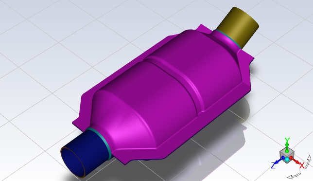
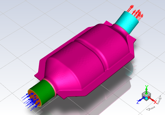
The catalytic converter modeled here is shown in Figure 3.6: Catalytic Converter Geometry for Flow Modeling. The nitrogen flows through the inlet with a uniform velocity of 125 m/s and 800K, passes through a pair of ceramic monolith substrates with square-shaped channels, and then exits through the outlet.

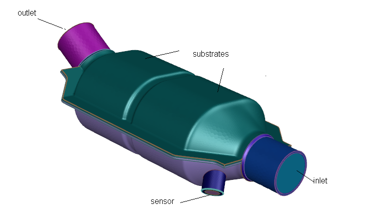
Figure 3.6: Catalytic Converter Geometry for Flow Modeling

While the flow in the inlet and outlet sections is turbulent, the flow through the substrates is laminar and is characterized by inertial and viscous loss coefficients along the inlet axis. The substrates are impermeable in other directions. This characteristic is modeled using loss coefficients that are three orders of magnitude higher than in the main flow direction.

3.5.4. Setup and Solution

The following sections describe the setup and solution steps for this tutorial:

3.5.4.1. Preparation

To prepare for running this tutorial:

Download the catalytic_converter.zip file here .
Unzip catalytic_converter.zip to your working directory.
The Discovery CAD file catalytic_converter.dsco can be found in the folder.
Use the Fluent Launcher to start Ansys Fluent.
Select Meshing in the top-left selection list to start Fluent in Meshing Mode.
Enable Double Precision under Options.
Set Meshing Processes and Solver Processes to 4 under Parallel (Local Machine).

3.5.4.2. Enable the Unified Topology Layer

The ability to separate physics settings from the mesh must be enabled before you begin the meshing workflow.

Open the Preferences dialog box.
File → Preferences...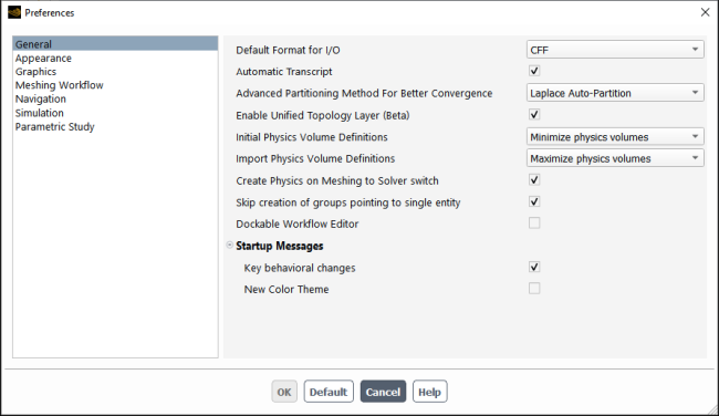
Enable the Enable Unified Topology Layer (Beta) option and disable the Create Physics on Meshing to Solver switch option in the General branch.
Click OK.

3.5.4.3. Meshing Workflow

Start the meshing workflow.
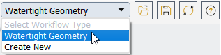
1. In the Workflow tab, select the Watertight Geometry workflow.
2. Review the tasks of the workflow.
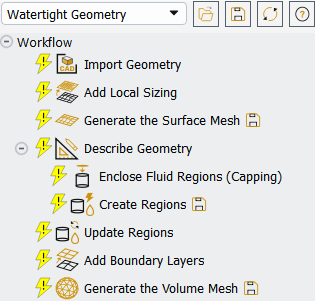
  Each task is designated with an icon indicating its state (for example, as complete, incomplete, etc. For more information, see Understanding Task States in the Fluent User's Guide). All tasks are initially incomplete and you proceed through the workflow completing all tasks. Additional tasks are also available for the workflow. For more information, see Customizing Workflows in the Fluent User's Guide.
Import the CAD geometry (catalytic_converter.dsco).
1. Select the Import Geometry task.
2. For File Format, keep the default setting of CAD.
3. For Units, keep the default setting as mm.
4. For File Name, enter the path and file name for the CAD geometry that you want to import (catalytic_converter.scdoc).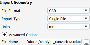
5. Select Import Geometry.
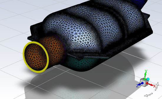
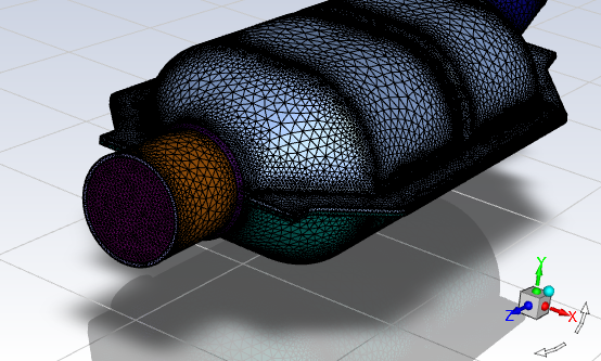
  This will update the task, display the geometry in the graphics window (Figure 3.7: The Imported CAD Geometry for the Catalytic Converter), and allow you to proceed onto the next task in the workflow.
  Figure 3.7: The Imported CAD Geometry for the Catalytic Converter
  
  Note: Alternatively, you can use the ... button next to File Name to locate the CAD geometry file, after which, the Import Geometry task automatically updates, displaying the geometry in the graphics window, and the workflow automatically progresses to the next task.
  Throughout the workflow, you are able to return to a task and change its settings using either the Edit button, or the Revert and Edit button. For more information, see Editing Tasks in the Fluent User's Guide.
Add local sizing.
1. In the Add Local Sizing task, you are prompted as to whether or not you would like to add local sizing controls to the faceted geometry.
  In this tutorial, we will add local sizing in and around the sensor, since that is an area where we require a more refined mesh. Later, we will apply settings for a coarser surface mesh elsewhere.
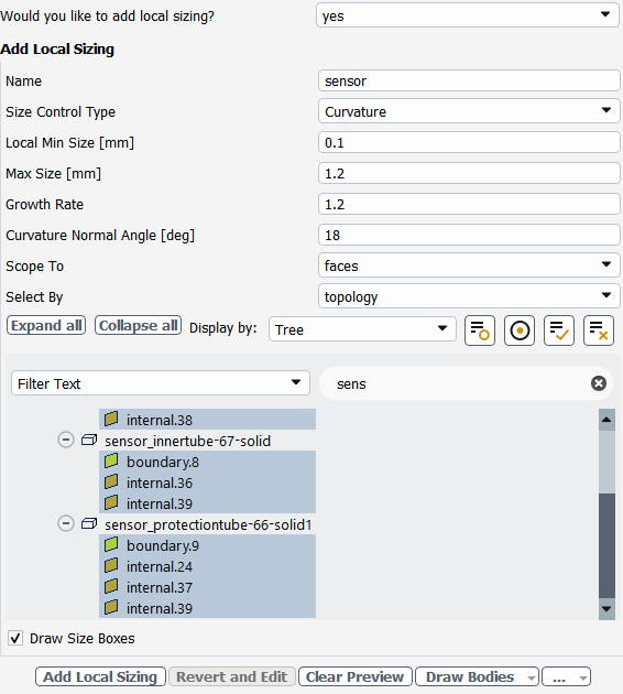
2. At the prompt for adding local sizing, select yes.
3. Specify Curvature for the Size Control Type.
4. Enter sensor for the Name of the size control.
5. Specify 0.1 for the Local Min Size.
6. Specify 1.2 for the Max Size
7. Select the child faces of the bodies in and around the sensor in the list, specifically, sensing_element-65-solid, sensor_innertube-67-solid, and sensor_protectiontube-66-solid1. Hold Ctrl while selecting the faces under each of the sensor bodies.
  Enter sens* into the Filter Text field to reduce the number of listed bodies.
8. Click Add Local Sizing to complete this task and proceed to the next task in the workflow.
Generate the surface mesh.
1. In the Generate the Surface Mesh task, you can set various properties of the surface mesh for the faceted geometry.
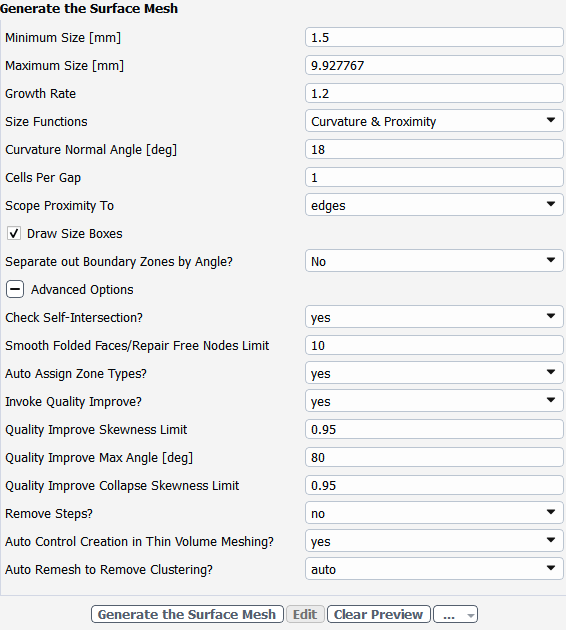
2. Specify 1.5 for the Minimum Size.
  Note: The red boxes displayed on the geometry in the graphics window are a graphical representation of size settings. These boxes change size as the values change, and they can be hidden by using the Clear Preview button.
3. Specify No for the Separate Out Boundary Zones by Angle? option.
4. Select Advanced Options to expose additional settings.
5. Specify 0.95 for the Quality Improve Skewness Limit.
6. Click Generate the Surface Mesh to complete this task and proceed to the next task in the workflow.
Describe the geometry.
When you select the Describe Geometry task, you are prompted with questions relating to the nature of the imported geometry.
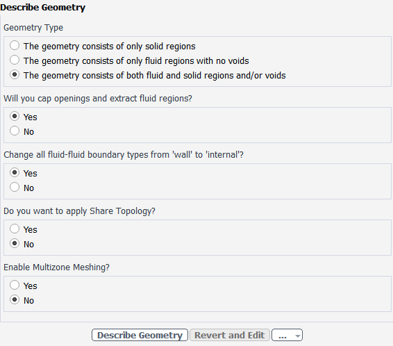
1. Select The geometry consists of both fluid and solid regions and/or voids option under Geometry Type, since this model contains both fluid and solids, and potential voids.
2. Select Yes for the Will you cap openings and extract fluid regions? prompt, since we plan on adding capping surfaces and extracting a fluid.
3. Select Yes for the Change all fluid-fluid boundary types from 'wall' to 'internal'? prompt, since we are modeling flow through the entire geometry, and any interior wall boundaries between potential fluid regions should be interior boundaries to allow the flow to pass.
  Remember that there are two regions within the catalytic converter that will ultimately represent porous regions.- surrounded by other non-porous fluid regions For now, we will consider all of these internal regions as fluid regions and change them accordingly in the Ansys Fluent solver.
4. Keep the rest of the default settings for this task.
5. Click Describe Geometry to complete this task and proceed to the next task in the workflow.
Cover any openings in your geometry.
Select the Enclose Fluid Regions (Capping) task, where you can cover, or cap, any openings in your geometry in order to later extract the enclosed fluid region.
1. Create a cap for the inlet.
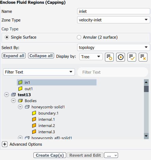
  1. Enter inlet for the Name of the capping surface to be assigned to the manifold's inlet.
  2. For the Zone Type, keep the default setting of velocity-inlet.
  3. Enter in into the Filter Text field and select in1 from the topology list.
    The graphics window indicates the selected items.
  4. Click Create Cap(s) to complete this task and proceed to the next task in the workflow.
    Once completed, this particular task will return you to a fresh task in order to assign additional capping surfaces, if necessary. We will proceed to assign a cap for the remaining opening and assign it to be an outlet.
2. Create a cap for the outlet.
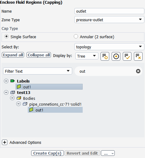
  1. Enter outlet for the Name of the capping surface to be assigned to the manifold's outlet.
  2. For the Zone Type, change the setting to pressure-outlet.
  3. Enter out into the Filter Text field and select out1 from the topology list.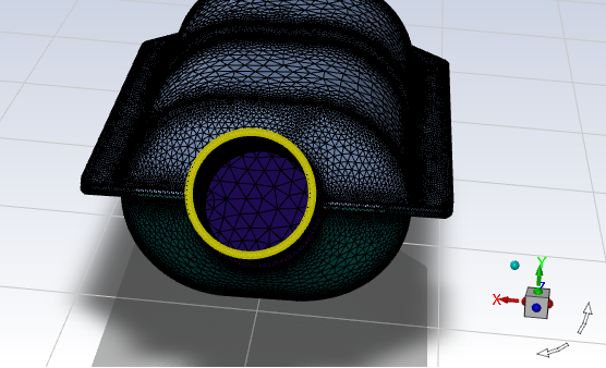
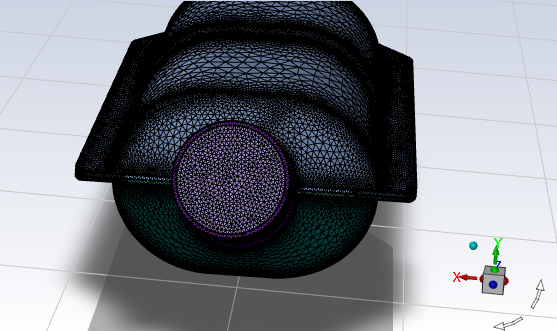
  4. Click Create Cap(s) to complete this task.
  Now, all of the openings in the geometry are covered.
Confirm and update the boundaries.
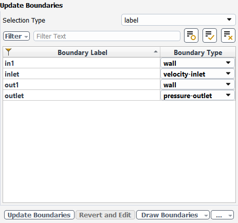
1. Select the Update Boundaries task, where you can inspect the mesh boundaries and confirm and change any designated boundaries accordingly. Ansys Fluent attempts to determine the correct arrangement of boundaries automatically.
2. Select label from the Selection Type drop-down list.
3. All the proposed boundaries are correct, so click Update Boundaries. and proceed to the next task.
Create the fluid region.
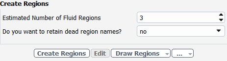
1. Select the Create Regions task, where you can determine the number of fluid regions that need to be extracted. Ansys Fluent attempts to determine the number of fluid regions to extract automatically.
2. For the Estimated Number of Fluid Regions, enter a value of 3.
  We anticipate that there will be fluid regions located at the inlet, the outlet, and the fluid region between the substrates.
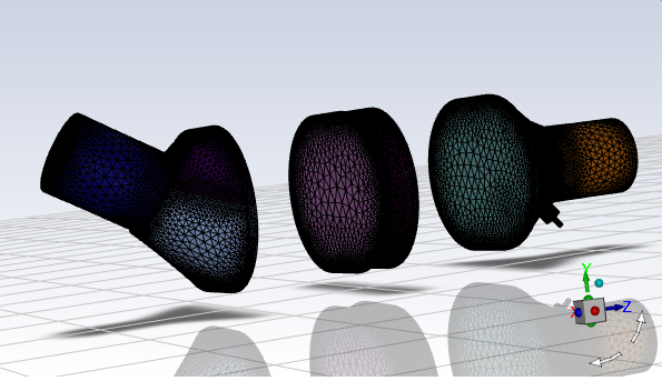
3. Click Create Regions.
  The extracted fluid regions are displayed in the graphics window.
Update your regions.
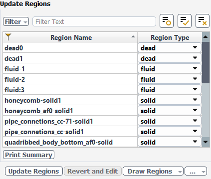
1. Select the Update Regions task, where you can review and change the tabulated names and types of the various regions that have been generated from your imported geometry, and change them as needed.
  We can see that the three fluid regions are defined, however, the two regions of the individual substrates are identified as solid regions. We can change their designations here in this task, and provide them with useful names.
2. Change the two substrate solid regions to be fluid regions, and rename them, in the table.
  1. Under Region Name, locate the honeycomb.solid1 region, double-click and rename the region to fluid:substrate:1.
  2. For that specific region, under Region Type, select fluid from the drop-down menu.
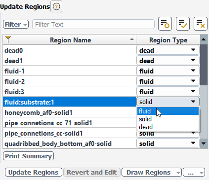
3. Repeat the procedure for the honeycomb_af0-solid1 region, renaming it to fluid:substrate:2.
4. Click Update Regions to update your settings.
Add boundary layers.
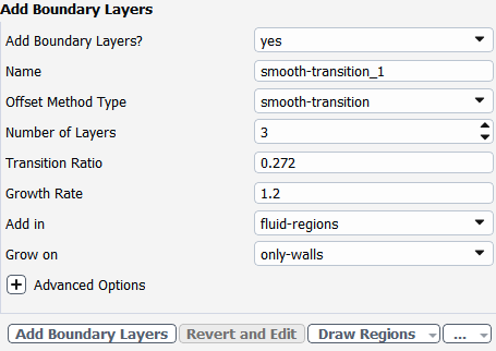
1. Select the Add Boundary Layers task, where you can set properties of the boundary layer mesh.
  For the Add Boundary Layers task, ensure yes is selected at the prompt as to whether or not you want to define boundary layer settings. In this task, you can define specific details for capturing the boundary layer in and around your geometry.
2. Keep the default settings, and click Add Boundary Layers.
Generate the volume mesh.
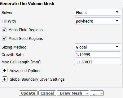
1. Select the Generate the Volume Mesh task, where you can set properties of the volume mesh itself.
2. Keep the default settings, and click Generate the Volume Mesh.
  Ansys Fluent will apply your settings and proceed to generate a volume mesh for the manifold geometry. Once complete, the mesh is displayed in the graphics window and a clipping plane is automatically inserted with a layer of cells drawn so that you can quickly see the details of the volume mesh.
  Note: You may receive the following warning after this step completes:
```
---- Warning --- Prism stair-step has occured in 6 location(s).
```
Check the mesh.
Mesh → Check
Save the mesh file (catalytic_converter.msh.h5).
File → Write → Mesh...
Switch to Solution mode.
Now that a high-quality mesh has been generated using Ansys Fluent in meshing mode, you can now switch to solver mode to complete the set up of the simulation.
We have just checked the mesh, so select Yes when prompted to switch to solution mode.

3.5.4.4. General Settings

Load the starting mesh file catalytic_converter.msh.h5. File → Read → Mesh...

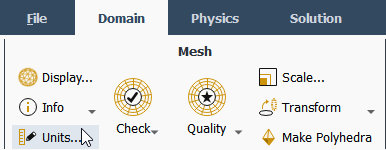
Set the units for length in the Set Units dialog box. Click Units... in the Domain ribbon tab (Mesh group box).

Domain → Mesh → Units...

This opens the Set Units dialog box.

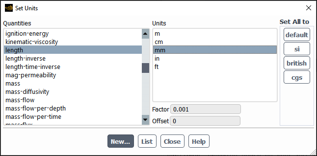
Select length under Quantities.
Select mm under Units.
Close the Set Units dialog box.
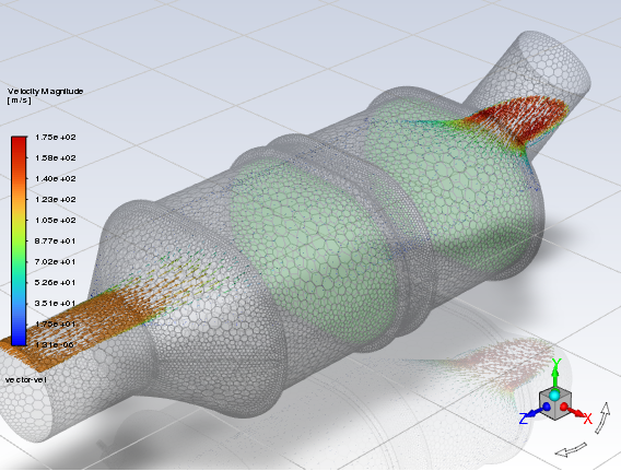
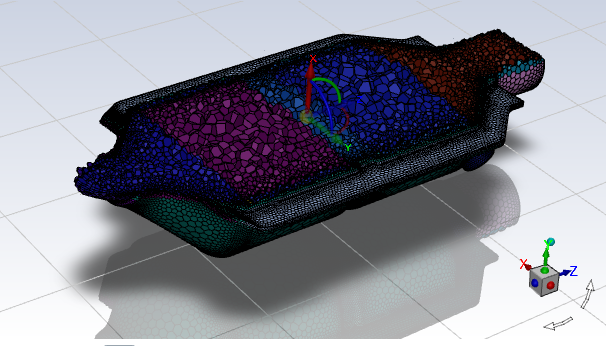
Examine the mesh.
Rotate the view and zoom in to get the display shown in Figure 3.8: Mesh for the Catalytic Converter Geometry in Fluent (Solver Mode).
Figure 3.8: Mesh for the Catalytic Converter Geometry in Fluent (Solver Mode)

3.5.4.5. Solver Settings

Retain the default solver settings.

Physics → General...

3.5.4.6. Models

Allow temperatures to be considered in the calculations by enabling the energy model.
You can enable the calculation of temperatures directly from the tree by right-clicking the Energy node and choosing On from the context menu.
Setup → Models → Energy On
Retain the default k-ω SST turbulence model.
You will use the default settings for the k-ω SST turbulence model, so you can enable it directly from the tree by right-clicking the Viscous node and choosing SST k-omega from the context menu.
Setup → Models → Viscous Model → SST k-omega

3.5.4.7. Materials

Add nitrogen to the list of fluid materials by copying it from the Fluent Database of materials.

Physics → Materials → Create/Edit...

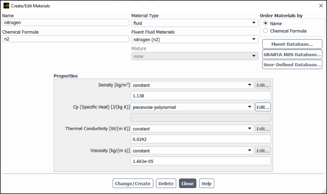
Click the Fluent Database... button to open the Fluent Database Materials dialog box.
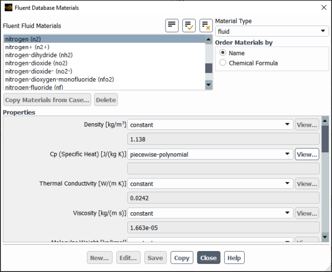
1. Select nitrogen (n2) in the Fluent Fluid Materials selection list.
2. Click Copy to copy the information for nitrogen to your list of fluid materials.
3. Close the Fluent Database Materials dialog box.
Click Change/Create and close the Create/Edit Materials dialog box.

3.5.4.8. Cell Zone Conditions

Define the physics for the non-porous fluid regions.
1. Right-click the fluid volume that was created by default and select Split into New Volume....
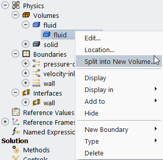
2. Enter porous-substrate-fluid for the Name of new volume. Select fluid:substrate:1 and fluid:substrate:2 in the Split fluid dialog box and click OK. Hold ctrl while selecting with the left mouse button.
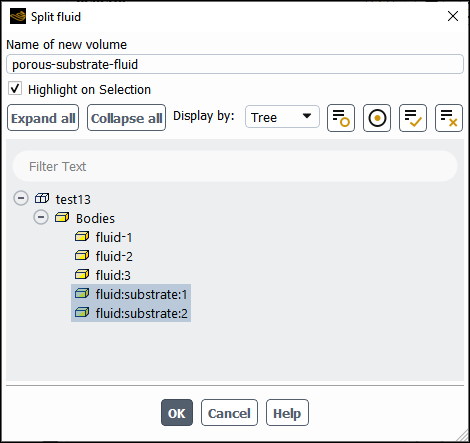
  As soon as you update the physics location and confirm, Fluent creates the necessary interfaces for the split fluid volumes.
3. Right-click the fluid physics volume and select Edit....
4. Select nitrogen in the Material Name drop-down, click Apply and close the Fluid dialog box.
Define the physics for the porous substrate fluid regions.
Setup → Physics → Volumes → fluid → porous-substrate -fluid Edit...
1. Enable Porous Zone and Laminar Zone, confirm that nitrogen is selected as the Material Name.
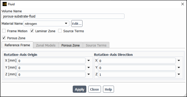
2. Click Apply and close the Fluid dialog box.

3.5.4.9. Boundary Conditions

Specify the conditions for the velocity inlet.
Setup → Physics → Boundaries → velocity-inlet → inlet Edit...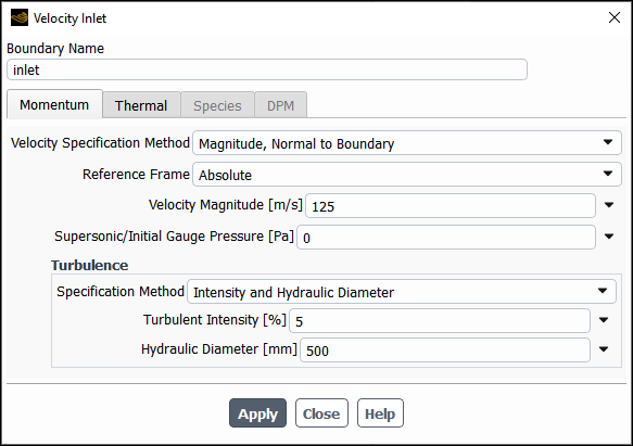
1. Enter 125 m/s for Velocity Magnitude.
2. In the Turbulence group box, select Intensity and Hydraulic Diameter from the Specification Method drop-down list.
3. Enter 5% for the Turbulent Intensity.
4. Enter 500mm for the Hydraulic Diameter.
5. Click the Thermal tab and enter 800 K for the Temperature of the incoming fluid.
6. Click Apply and close the Velocity Inlet dialog box.
Specify the conditions for the pressure outlet.
Setup → Physics → Boundaries → pressure-outlet → outlet Edit...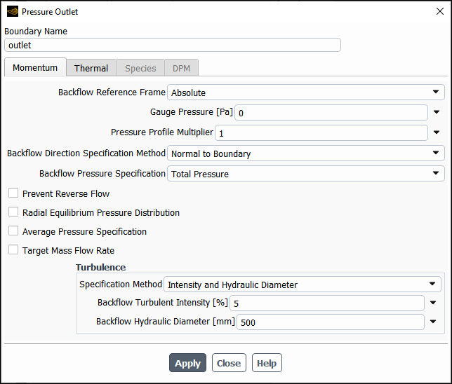
1. Retain the default setting of 0 for Gauge Pressure.
2. In the Turbulence group box, select Intensity and Hydraulic Diameter from the Specification Method drop-down list.
3. Retain the default value of 5% for the Backflow Turbulent Intensity.
4. Enter 500 mm for the Backflow Hydraulic Diameter.
5. Click the Thermal tab and enter 800 K for the Backflow Total Temperature of the outgoing fluid.
6. Click Apply and close the Pressure Outlet dialog box.
Retain the remaining default (wall and interior) boundary conditions.

Note: With the conditions specifications complete, it is beneficial to collapse the Physics branch again, reducing the size of the tree.

3.5.4.10. Solution

Specify the discretization schemes.
Solution → Solution → Methods...

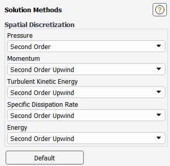
Retain the default settings.
Enable the plotting of the mass flow rate at the outlet.
Solution → Reports → Definitions → New → Surface Report → Mass Flow Rate
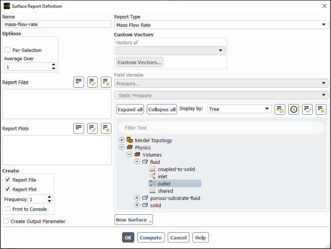
1. Enter mass-flow-outlet for the Name of the surface report definition.
2. Enter Outlet in the Filter Text field, collapse the Geometry branch, expand the Physics branch and select outlet.
3. Click OK to save the surface report definition settings and close the Surface Report Definition dialog box.
Initialize the solution.
Solution → Initialization
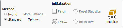
1. Select Standard under Method.
  Warning: Standard is the recommended initialization method for porous media simulations. The default Hybrid method does not account for the porous media properties, and depending on boundary conditions, may produce an unrealistic initial velocity field. For porous media simulations, the Hybrid method should only be used when the Maintain Constant Velocity Magnitude option is enabled in the Hybrid Initialization dialog box.
2. Click Options... to open the Solution Initialization task page, which provides access to further settings.
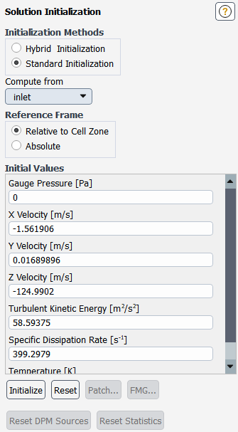
  1. Select inlet from the Compute from drop-down list in the Solution Initialization task page.
  2. Retain the default settings for standard initialization method.
  3. Click Initialize.
Save the case file (catalytic_converter_UTL.cas.h5).
File → Write → Case...
Start the calculation.
Solution → Run Calculation → Run Calculation...
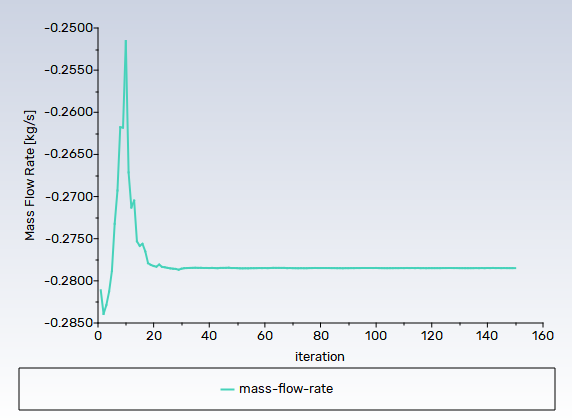
1. Enter 150 for No. of Iterations.
2. Click Calculate to begin the iterations.
  The mass flow rate graph flattens out, as seen in Figure 3.9: Mass Flow Rate History. Since the mass flow rate has stabilized after 150 iterations, the solution can be said to have reached convergence.
  Figure 3.9: Mass Flow Rate History
Save the case and data files (catalytic_converter_UTL.cas.h5 and catalytic_converter_UTL.dat.h5).
File → Write → Case & Data...

3.5.4.11. Postprocessing

Display the wall surfaces.
Results → Graphics → Mesh... → New...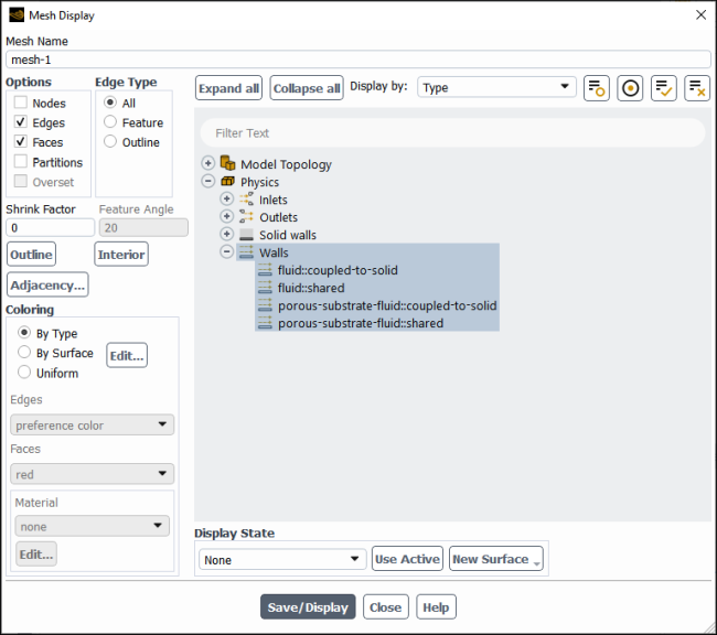
1. Select Edges and Faces in the Options group box.
2. Select Outline in the Edge Type group box.
3. Select Type from the Display By drop-down list.
4. Expand Wall under Physics and select all the children.
5. Click Save/Display and close the Mesh Display dialog box.
Create a surface passing through the geometry for postprocessing purposes.
Results → Surface → Create → Plane...
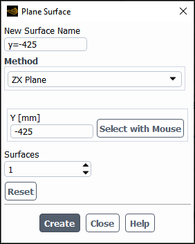
1. Enter y=-425 as the New Surface Name.
2. Select ZX Plane from the Method drop-down list.
3. Enter -425 for Y.
4. Click Create.
Create cross-sectional planes at locations throughout the domain: in the inlet prior to the first substrate, within the first substrate, in the fluid zone between the substrates, within the second substrate, and just after the second substrate in the outlet.
Results → Surface → Create → Plane...
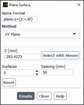
1. Skip entering a New Surface Name because the system will automatically create meaningful names when multiple are created at once.
2. Select XY Plane from the Method drop-down list.
3. Enter 185 for Z.
4. Enter 5 for Surfaces and 50 for Spacing.
5. Click Create.
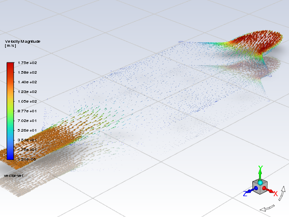
Display velocity vectors on the y=-425 surface (Figure 3.10: Velocity Vectors Through the Interior).
Results → Graphics → Vectors → New...
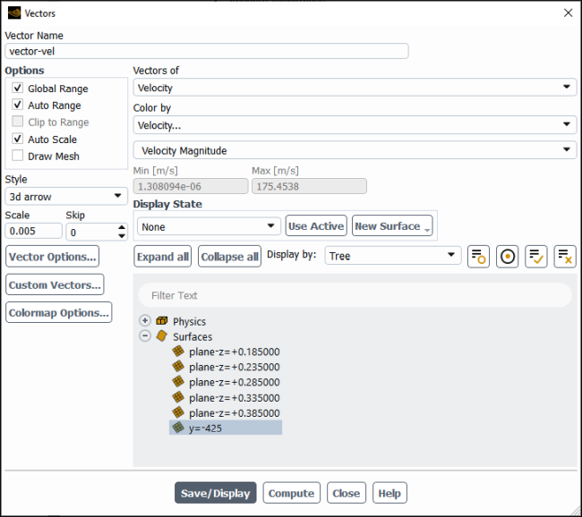
1. Enter vector-vel for Vector Name.
2. Disable Global Range under Options.
3. Assign a value of 0.005 for Scale.
4. Select y=-425 in the Surfaces selection list.
5. Click Save/Display and close the Vectors dialog box.
6. Rotate the view and adjust the magnification to get the display shown in Figure 3.10: Velocity Vectors Through the Interior.
  Figure 3.10: Velocity Vectors Through the Interior
  
  The flow pattern shows that the flow enters the catalytic converter as a jet, with recirculation on either side of the jet. As it passes through the porous substrates, it decelerates and straightens out, and exhibits a more uniform velocity distribution. This allows the metal catalyst present in the substrates to be more effective.
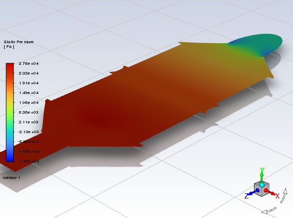
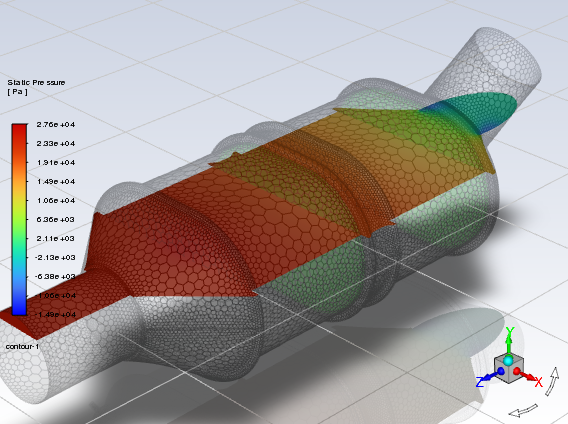
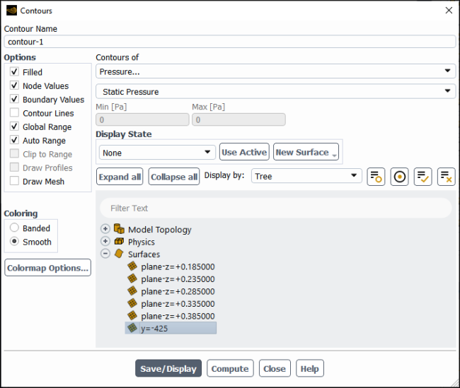
Display filled contours of static pressure on the interior plane (Figure 3.11: Contours of Static Pressure Through the Interior).
Results → Graphics → Contours → New...
1. Enter contour-pressure for Contour Name.
2. Make sure that Filled, Node Values, and Boundary Values are enabled in the Options group box.
3. Make sure that Pressure... and Static Pressure are selected from the Contours of drop-down lists.
4. Select y=-425 in the Surfaces selection list.
5. Click Save/Display and close the Contours dialog box.
The pressure changes rapidly in the middle section, where the fluid velocity changes as it passes through the porous substrates. The pressure drop can be high, due to the inertial and viscous resistance of the porous media.
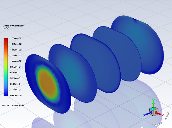
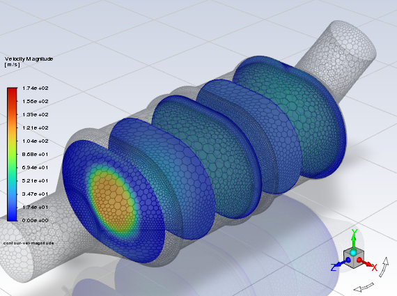
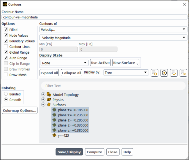
Figure 3.11: Contours of Static Pressure Through the Interior
Display filled contours of the velocity magnitude on the z=185=0, z=185=50, z=185=100, z=185=150, and z=185=200 surfaces (Figure 3.12: Contours of Velocity Magnitude at z=185, z=230, z=280, z=330, and z=375).
Results → Graphics → Contours → New...
1. Enter contour-vel-mag for Contour Name.
2. Ensure that Filled, Node Values, and Boundary Values are enabled in the Options group box.
3. Disable Global Range in the Options group box.
4. Select Velocity... and Velocity Magnitude from the Contours of drop-down lists.
5. Select z=185=0, z=185=50, z=185=100, z=185=150, and z=185=200 in the Surfaces selection list, and deselect all others.
6. Click Save/Display and close the Contours dialog box.
Figure 3.12: Contours of Velocity Magnitude at z=185, z=230, z=280, z=330, and z=375

The velocity profile becomes more uniform as the fluid passes through the porous media. The velocity is higher at the center (the area in red) just before the nitrogen enters the substrates and then decreases as it passes through and exits the second substrate. The area in green, which corresponds to a moderate velocity, increases in extent.
Create scene graphics objects for each postprocessing display to visualize them within the context of the geometry.
Results → Scene New...
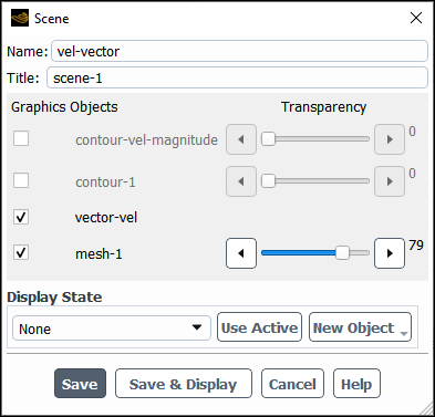
1. Enter velocity-vectors for the Name.
2. Select vector-vel and mesh-1 and increase the transparency on mesh-1 to 79 using the slider.
3. Click Save & Display.
4. Right-click the newly-created velocity-vectors scene object in the tree and select Copy....
5. Name the copied object pressure-contour, deselect vector-vel and select contour-pressure.
6. Repeat these steps for contours of velocity magnitude, creating a scene object named velocity-magnitude-contours.
Figure 3.13: Scene of Velocity Vectors

Figure 3.14: Scene of Pressure Contours

Figure 3.15: Scene of Velocity Magnitude Contours
Save the case and data file.
File → Write → Case & Data...

3.5.5. Summary

In this tutorial, you learned how to set up and solve a problem involving gas flow through porous media in Ansys Fluent. You also learned how to perform appropriate postprocessing. Flow non-uniformities were easily identified through images of velocity vectors and pressure contours.