


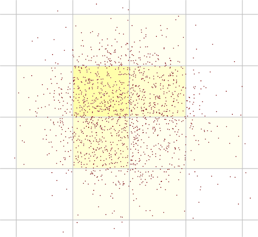
The DEM-CFD coupling method was developed for the ideal case in which the particles are smaller than the CFD cells (Figure 6.1: Schematic representation of many particles with volumes smaller than CFD cells, with volume fraction values calculated by represented as cell colors. In this situation the volume fraction distribution is realistic.), so that the particulate phase volume fraction of a cell can be calculated as:
 | (6–12) |
where  is the computational cell volume,
  is the particle volume and N is the number of particles
whose centroids lie inside the cell.
is the particle volume and N is the number of particles
whose centroids lie inside the cell.
Figure 6.1: Schematic representation of many particles with volumes smaller than CFD cells, with volume fraction values calculated by represented as cell colors. In this situation the volume fraction distribution is realistic.
Equation 6–12 is accurate as long as
 . As the relative sizes of the particles increase compared to the sizes of
the cells, however, the discrete representation of particles in the DEM domain cause Equation 6–12 to lose accuracy when mapping solid
volume to the CFD domain, as represented by:
. As the relative sizes of the particles increase compared to the sizes of
the cells, however, the discrete representation of particles in the DEM domain cause Equation 6–12 to lose accuracy when mapping solid
volume to the CFD domain, as represented by:
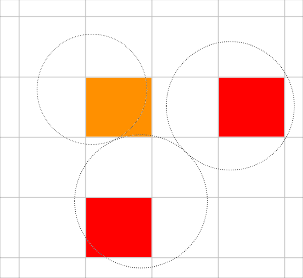
Figure 6.2: Schematic representation of 3 particles with volumes greater than CFD cells, with volume fraction values calculated by represented as cell colors. In this situation the volume fraction distribution is unrealistic - there are cells with more than 100% of solid volume while neighboring cells are empty of solid volume.
In order to refrain from sending unrealistic values of solid volume fraction to the CFD domain, in which the flow is described following an Eulerian approach, a subsequent step that redistributes the solid phase is performed. Rocky provides two options to perform this Lagrangian-to-Eulerian (L-E) mapping: uniform distribution and volumetric diffusion.
Note: The mapped information covers the solid fraction, interaction forces and exchanged heat amounts.
The uniform distribution is used when the is set to Uniform Distribution in the in Rocky.
This method works by considering an averaging radius value  that defines a new cell, herein called "super-cell", as shown in
Figure 6.3: Schematic depiction of a super-cell and its averaging radius.. This super-cell is formed by the original cell and all
the neighboring cells having their centroids located inside a sphere with radius equal to
that defines a new cell, herein called "super-cell", as shown in
Figure 6.3: Schematic depiction of a super-cell and its averaging radius.. This super-cell is formed by the original cell and all
the neighboring cells having their centroids located inside a sphere with radius equal to
 .
.
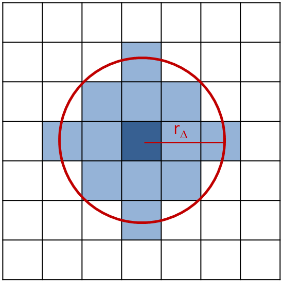
In this mapping, the averaging is performed considering a uniform distribution over the cells contained inside the super-cell. The idea of the mapping is to distribute the volume fraction and interaction forces of the central cell equally to all cells composing the super-cell.
In the uniform distribution, L-E mapping, the averaging radius, , is a user input and may be given either as an absolute value or as a
fraction of the maximum particle diameter according to the parameter Averaging Radius Type in the Fluent Two-Way Coupling settings in Rocky.
In order to obtain the contribution to the volumetric fraction for all cells forming a super-cell, the volume of all particles located at the center of the super-cell are summed and divided by the total volume of the super-cell:
 | (6–13) |
where  is the volume fraction contribution for all cells inside the super-cell,
 is the volume of each particle,
  is the number of particles that have their centroids located inside the
center cell of the super-cell and, finally,
VSC
is the volume of the super-cell, computed according to:
is the number of particles that have their centroids located inside the
center cell of the super-cell and, finally,
VSC
is the volume of the super-cell, computed according to:
 | (6–14) |
where  and
and  are, respectively, the number and the volume of the cells composing a
super-cell.
are, respectively, the number and the volume of the cells composing a
super-cell.
Figure 6.4: Addition of contributions of two overlapped super-cells when uniform averaging scheme is used: (a) contribution for the super-cell delimited by the red circle, (b) contribution for the super-cell delimited by the orange circle, (c) added contributions from the two previous super-cells.
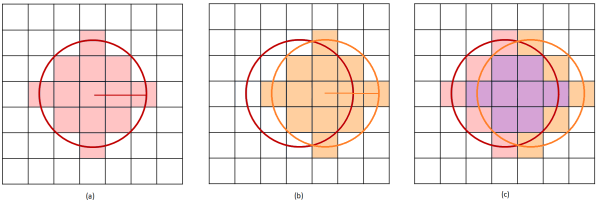
This procedure is repeated for all NT cells in the fluid domain, i.e., NT super-cells are generated and the contribution of each one of them is added to obtain the final volume fraction of particles at each one of the NT cells in the fluid domain. shows an example of the addition of contributions of two overlapped super-cells.
In order to obtain the quantities that have to be sent to the CFD solver, this same averaging process is also performed for the total interaction force as well as the heat transfer rate with the fluid.
The uniform distribution tends to perform sub-optimally under the following circumstances:
Heterogeneous meshes. By default the super-cell is 3.5 times larger than the largest cell of the mesh. If the mesh contains regions that are heavily refined compared to its largest cells, the computational cost of searching cells inside the perimeter of the super-cell increases at these regions due to the increased amount of cells that may fit inside the perimeter.
Internal boundaries. To determine which cells are part of the super-cell, the search algorithm considers only the spatial location of the cells and disregards its topological information, as the latter is too computationally complex for the algorithm to handle. In corner cases of cells separated by a thin internal boundary, this may lead to volume fraction being "leaked" across the boundary by the mapping process if the cells are small enough (and positioned close enough) to eventually fit inside the super-cell at the same time.
Note: Using smaller values for the supercell perimeter may impact the mapping quality at the largest cells of the mesh.
To overcome these issues, the (section Volumetric diffusion L-E mapping) has been implemented.
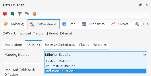
The volumetric diffusion L-E mapping is enabled when the Mapping Method is set to Volumetric Diffusion in the in Rocky. This method works by solving iteratively a discretized diffusion equation on the CFD mesh. With each iteration, calculated amounts of exceeding solid volume (and other physical quantities related to the particle phase as well) are exchanged between each cell and its immediate neighbors. These amounts are proportional to the difference of values between the cell and its immediate neighbors, and are tuned by automatic detection of individual optimal diffusion coefficients for each cell. Iterations are repeated until a target maximum volume fraction is achieved over the mesh, or a maximum number of iterations is reached.
The next sections explain the method in detail.
The volumetric diffusion L-E mapping handles the problem of smoothing the distribution
of solid volume as a process of molecular diffusion in a fluid medium. Fick's second law
of diffusion predicts how diffusion causes the concentration  of a given substance to change as time passes in an isotropic
homogeneous medium:
of a given substance to change as time passes in an isotropic
homogeneous medium:
 | (6–15) |
where D is the diffusion coefficient for  in the medium.
In a discrete homogeneous mesh, the continuous Laplacian can be expressed as a graph
Laplacian. Then for any given cell  of the mesh, can be expressed as:
 | (6–16) |
where  is the substance concentration at cell i, and
 is the set of all cells that are immediate neighbors of
  .
.
Equation 6–16 can be solved numerically by an
explicit iterative method. For this numerical solution a unit time step can be assumed,
since an accurate transient solution is not of interest - but only the final state in
which the concentration  has been diffused after enough iterations. The explicit iterative form
of equation is:
has been diffused after enough iterations. The explicit iterative form
of equation is:
 | (6–17) |
Equation 6–17 offers an iterative approach to smooth an initial distribution of volumetric fraction values in homogeneous meshes. For heterogeneous meshes, in order to conserve the total amount of solid in the solution domain as the iterative process evolves, the diffusion coefficient D can be expressed as being inversely proportional to the volume of the cell. can then be adapted to:
 | (6–18) |
where  is a constant.
Equation 6–18 shows that the smaller the
 value, the longer it takes to smooth the solid volume field iteratively.
Therefore
value, the longer it takes to smooth the solid volume field iteratively.
Therefore  is desired to be as large as possible; however a maximum limit must be
defined for
is desired to be as large as possible; however a maximum limit must be
defined for  to guarantee the stability of the iterative process.
It was determined heuristically that the following value of  provides a satisfactory compromise between the speed and the stability
of the method in homogeneous meshes:
provides a satisfactory compromise between the speed and the stability
of the method in homogeneous meshes:
Note: This criteria was deduced by considering a regular unbounded mesh ? the shape of
the cells is irrelevant ? containing a regular distribution of volume, where half of
its cells are filled with the same amount of solid volume and half are empty. After
one iteration, this value of causes all cells of the mesh to contain the same amount of solid
volume.
 | (6–19) |
where  is the minimum cell volume found among all cells of the mesh and
Nmax
is the maximum number of immediate neighbors found among all cells of the mesh.
is the minimum cell volume found among all cells of the mesh and
Nmax
is the maximum number of immediate neighbors found among all cells of the mesh.
Note: In fact, forcing a unique value of tuned to the smaller cell of a heterogeneous mesh would impose an
unnecessary burden to larger cells whose L-E mapping could be performed faster with
their own larger values of .
For heterogeneous meshes, Rocky takes advantage of the fact that  does not need to be the same for all cells of the mesh. Instead, the
only requirement is that each pair of cells that undergo a transfer of solid volume must
agree on the same
does not need to be the same for all cells of the mesh. Instead, the
only requirement is that each pair of cells that undergo a transfer of solid volume must
agree on the same  . Rocky uses this fact to automatically determine optimum diffusion
constants for each cell as:
. Rocky uses this fact to automatically determine optimum diffusion
constants for each cell as:
 | (6–20) |
where  is the number of immediate neighbors of cell
  .
.
Then in Equation 6–18 , the same value of
 must be used whenever the same pair of cells undergo a solid transfer.
Since each cell has its own
must be used whenever the same pair of cells undergo a solid transfer.
Since each cell has its own  - which happens to be the maximum allowable value for the cell to
undergo stable solid exchanges - the smaller value of the pair must be chosen. Considering
this requirement, Equation 6–18 can be
rewritten to:
- which happens to be the maximum allowable value for the cell to
undergo stable solid exchanges - the smaller value of the pair must be chosen. Considering
this requirement, Equation 6–18 can be
rewritten to:
 | (6–21) |
where  is the value of
  for an immediate neighbor of the cell
  .
.
Equation 6–21 is the basis of the iterative algorithm implemented by Rocky. With each iteration, Rocky applies this algorithm to all cells of the CFD domain to calculate new volume fraction values. Iterations are repeated until the stop criteria described in section Operation are met.
Prior to starting a simulation in which the method has been chosen, Rocky calculates and stores the following information:
Sets of immediate neighbors of all cells of the mesh.
Diffusion constants (
 ) of all cells of the mesh according to Equation 6–20 .
Every time the L-E mapping must be performed during the simulation, Equation 6–21 is applied to all cells of the mesh to achieve a smoothed state of the solid volume distribution. This action comprises one iteration of the method. Rocky then decides if more iterations are required based on the following parameters that are set by the user under the Fluent Two-Way Coupling settings:
Maximum Volume Fraction Target - Desired maximum volume fraction over the mesh (default 65%). After each iteration the maximum volume fraction is queried over the mesh and, if no greater than the Maximum Volume Fraction Target , the mapping is declared finished.
Maximum Iterations - Maximum number of iterations that must be performed (default 500). If the number of performed iterations exceeds this value, the iterative process terminates in order for the solid volume distribution to be sent to Fluent.
Decomposition Factor - The Volumetric Diffusion algorithm may face problems when dealing with heterogeneous cases, either by different particle sizes in a homogenous mesh or by the same particle sizes in a heterogeneous mesh. This is because, the volumetric limiter is a global stopping criterion for a local, cell-based, solid fraction property. In other words, if a region of the mesh has a solid fraction > volumetric limiter it will force the diffusion to carry on even though some regions already have achieved the criteria solid fraction ≤ volumetric limiter. A new strategy was developed, in which only the regions that are above a certain level of volume fraction will have diffusion. A new parameter named Decomposition Factor was created, enabling the control of it. This parameter splits the quantities to be diffused, e.g. solid fraction, into parts x and y, where x is the quantity below the Decomposition Factor * Solid Fraction Target and y is the quantity to be diffused. Using this strategy we gain local control over the quantities, in such a way that a variable is not diffused when it is below the limit.
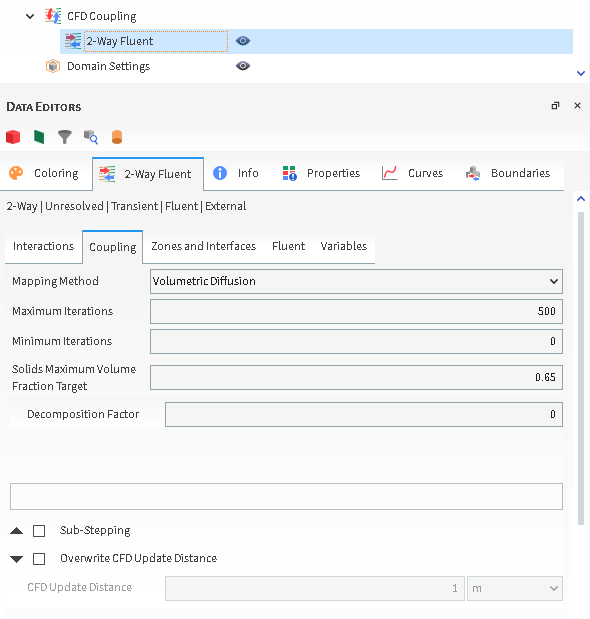
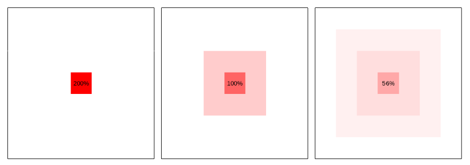
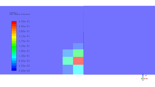
Figure 6.6: Representation of 2 iterations of the volumetric diffusion L-E mapping over a regular two-dimensional Cartesian mesh containing in its center cell a particle whose volume is two times greater than the cell's volume. illustrates the application of the with a default Maximum Volume Fraction Target of 65% to a regular two-dimensional Cartesian mesh containing in its center cell a particle whose volume is two times greater than the cell's volume. After two iterations the mapping is complete with a maximum solid volume fraction of 56% over the whole mesh.
Figure 6.6: Representation of 2 iterations of the volumetric diffusion L-E mapping over a regular two-dimensional Cartesian mesh containing in its center cell a particle whose volume is two times greater than the cell's volume.
Section Formulation describes how the smooths a field of solid volume fraction values. A similar approach is considered for mapping force- and thermal-related quantities, with the following considerations over the exchange of values between a cell and its neighbors.
Forces are weighted by the specific mass of the fluid contained in the cells at the moment the mapping is performed. The iterative equation for mapping forces is:
Note: A similar equation applies to mapping time derivatives of forces.
 | (6–22) |
where  is a force component at cell i.
Note: The L-E mapping is performed for each force component independently
Heat amounts are weighted by the volumetric heat capacity of the fluid contained in the cells at the moment the mapping is performed. The iterative equation for mapping heat amounts is:
Note: A similar equation applies to mapping time derivatives of heat amounts.
 | (6–23) |
Lastly, the iterations of force- and thermal-related quantities are coupled with the iterations of the solid volume mapping. Consequently there are no maximum target values for these quantities.
The volumetric diffusion L-E mapping can be further tuned in two-way coupled setups that contain more than one fluid zone by selecting what fluid zones are part of the mapping.
Note: The selection of the fluid zones is performed in Rocky via the Fluent Two- Way settings, Zones and Interfaces tab, Coupling Fluid Cell Zones section.
The L-E mapping does not happen in fluid zones that are not selected, increasing the computational efficiency of simulations where particles are known to never reach such zones.
Setups that contain moving meshes connected through sliding interfaces are supported by the L-E mapping algorithm.
Note: When setting up the simulation, the user must select which interfaces the volumetric diffusion L-E mapping is allowed to map across. The selection of the interfaces is performed in Rocky via the Fluent Two-Way settings, Zones and Interfaces tab, Mapping Cell Zone Interfaces section.
In order to correctly apply the L-E mapping across sliding interfaces, Rocky keeps a further list of neighbors that are in contact through the interfaces, as well as updated diffusion constants for nearby cells. The volumetric diffusion L-E mapping then honors the user selection of interfaces by adding this temporary set of neighbors to the static set of neighbors that was queried initially for all meshes individually.
Note: This information is constantly updated during the simulation as meshes move relative to each other.
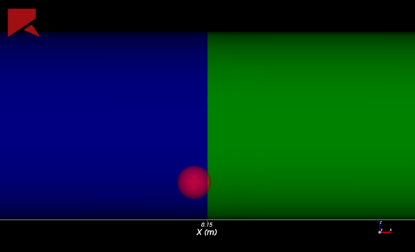
Consequently the volumetric diffusion L-E mapping distributes solid volume (and other physical quantities as well as per section Mapping other physical quantities) across the sliding interfaces that were selected by the user, while interfaces that were not selected behave as barriers to the mapping. For illustrating this concept, consider , which represents a particle near to the sliding interface between two meshes that rotate relative to each other.
If the sliding interface is selected under Mapping Cell Zone Interfaces in the UI, the volumetric diffusion L-E mapping expands solid volume towards the mesh at the other side of the interface as well Figure 6.8: Resulting volume fraction distribution when the situation represented by Figure 6.6 is mapped with the sliding interface selected under Mapping Cell Zone Interfaces.. This is the indicated setting when particles are intended to move freely through the sliding interface in the simulation, as the fluids at both sides of the interface are supposed to be equally disturbed by the solid volume.
Figure 6.8: Resulting volume fraction distribution when the situation represented by Figure 6.6 is mapped with the sliding interface selected under Mapping Cell Zone Interfaces.
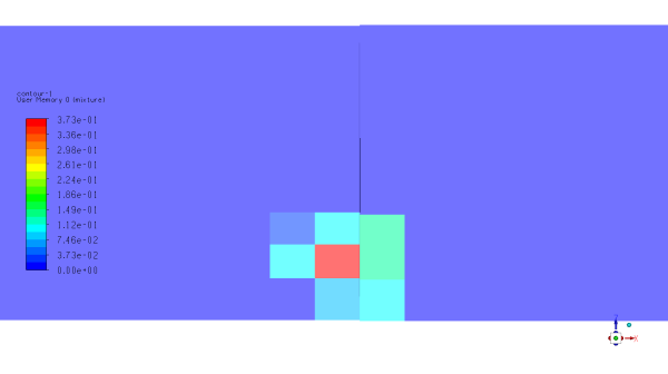
If the sliding interface is not selected under Mapping Cell Zone Interfaces in the UI, the mapping does not expand solid volume across the interface Figure 6.9: Resulting volume fraction distribution when the situation represented by Figure 6.6 is mapped with the sliding interface not selected under Mapping Cell Zone Interfaces. This is the indicated setting when the interface is intended to act as a free gateway for fluids in the CFD domain while blocking particles in the DEM domain.
Figure 6.9: Resulting volume fraction distribution when the situation represented by Figure 6.6 is mapped with the sliding interface not selected under Mapping Cell Zone Interfaces
Note: Typical examples are DEM-CFD coupled simulations containing geometries that act as sieves.
For the Diffusion and Advection of DEM quantities, when the Diffusion Equation is selected for Mapping Method, then it solves a diffusion equation to perform the mapping and smoothing of the volume fraction variables (particles volume fraction and particles volume fraction variation due to particles entering and leaving the domain) and a pure advection equation to all other quantities. This way all other mapped quantities (averaged particle quantities, momentum and energy sources, for example) are all distributed according the volume fraction distribution.
For the particle volume fraction variables, a simple diffusion equation is solved, given:
 | (6–24) |
where  is the particle fraction,
  is a pseudo time (as the diffusion equation is solved using its unsteady
form), and
is a pseudo time (as the diffusion equation is solved using its unsteady
form), and  is the volume fraction diffusion coefficient.
The initial condition is defined by the calculation of the particle volume on each cell. This is done simply by computing the ratio between the sum of the volume of particles inside each cell (determined solely by the particle centroid) and the cell volume. This can lead to volume fractions even larger than 1. The unsteady diffusion equation is then solved over time until the maximum volume fraction in the domain reaches the target volume fraction or the maximum number of time steps, both user-defined parameters. A unit pseudo-time step is assumed for the solution.
For all other quantities, a pure advection equation is solved:
 | (6–25) |
where  represents any of the additional variables mapped (averaged particles
velocity, temperature, momentum and energy sources, for example), and
represents any of the additional variables mapped (averaged particles
velocity, temperature, momentum and energy sources, for example), and  is the velocity computed using the diffusion of volume fraction. Using this
velocity, and solving the advection equation for the same number of time steps used in the
diffusion equation, we guarantee that all additional quantities are transported in the same
amount and in the same direction as the particle volume fraction. Generating a consistent
distribution of all quantities. The initial condition for all additional quantities mapped
is also computed using the accumulated values of each variable in the cells the particle
centroid is located
is the velocity computed using the diffusion of volume fraction. Using this
velocity, and solving the advection equation for the same number of time steps used in the
diffusion equation, we guarantee that all additional quantities are transported in the same
amount and in the same direction as the particle volume fraction. Generating a consistent
distribution of all quantities. The initial condition for all additional quantities mapped
is also computed using the accumulated values of each variable in the cells the particle
centroid is located
The equations are discretized using a central-difference spatial discretization scheme and a first order implicit time discretization. The advection term uses a first order upwind discretization. Information about these methods can be found in the Ansys Fluent Theory Guide, Release 2025R1, sections 24.3.1 and 24.3.2.
For the Back-Diffusion of Fluid and Flow Quantities, when diffusing/advecting DEM quantities in the DEM-CFD coupling, we extend the influence of the particles to a region that is usually larger than the particle sizes. So, the influence of the particle, which in the traditional Eulerian approach is submesh in scale, extends to a larger portion of the domain. The other way round should be true as well. The fluid properties and flow quantities used to compute the fluid-particle interactions should include information from the entire region affected by the presence of the particle, not only of the position where the particle centroid is located.

The Back-Diffusion method uses the same approach as the pure-advection of the DEM quantities applied in the Diffusion Solution mapping scheme, but using the inverse of the volume fraction diffusion velocity as the advection velocity, to compute a volume fraction weighted transport of the fluid properties and flow quantities at the position where the particles are located. So, assuming that a (large) particle had its volume diffused (as volume fraction) to 5 layers of cells around the central cell (where its centroid is located), the fluid/flow values of at the cell where the particle is located will be an average value of all these 5 layers of cells, with a smaller contribution of the cells farther away from the center cell than the ones closer to it.