


This tutorial includes:
- 36.1. Tutorial Features
- 36.2. Overview of the Problem to Solve
- 36.3. Preparing the Working Directory
- 36.4. Defining and Obtaining a Solution for the Steady-state Case
- 36.5. Defining and Obtaining a Solution for the Time Integration Solution Method Case
- 36.6. Defining and Obtaining a Solution for the Harmonic Balance Solution Method Case
- 36.7. Postprocessing the Blade Flutter Solution
In this tutorial you will learn about:
|
Component |
Feature |
Details |
|---|---|---|
|
CFX-Pre |
User Mode |
General mode |
|
Analysis Type |
Transient Blade Row | |
|
Fourier Transformation Pitch Change Model | ||
|
Time Integration Solution Method | ||
|
Harmonic Balance Solution Method | ||
|
Fluid Type |
Air Ideal Gas | |
|
Domain Type |
Multiple Domains | |
|
Rotating Frame of Reference | ||
|
Turbulence Model |
Shear Stress Transport | |
|
Heat Transfer |
Total Energy | |
|
Boundary Conditions |
Inlet (Subsonic) | |
|
Outlet (Subsonic) | ||
|
Wall (Counter Rotating) | ||
|
Mesh Motion |
Periodic Motion | |
|
Sliding Mesh | ||
|
CFD-Post |
Plots |
Contour |
|
Isosurface | ||
|
Vectors | ||
|
Transient Blade Row Expansion |
The goal of this tutorial is to set up transient blade row blade flutter simulations using
both time integration and harmonic balance transient methods in combination with the Fourier
Transformation pitch change model. An integral step of blade flutter modeling is the calculation
of the aerodynamic damping factor as a function of the possible nodal diameters (radial lines of
symmetry around the circumference) for the component being modeled. When the number of passages
in the component is an integer multiplier of the nodal diameter ( ), the number
of blade passages required to model a given nodal diameter can be
substantially reduced by using the rotational periodic boundary conditions.
This eliminates the need to model the full component. By using the
Fourier Transformation model, the number of passages required can
be kept to a minimum of two for all nodal diameters. The Harmonic balance transient method and the Fourier Transformation pitch
change model can each cut solution time independently; when combined, the solution time is
further reduced.
), the number
of blade passages required to model a given nodal diameter can be
substantially reduced by using the rotational periodic boundary conditions.
This eliminates the need to model the full component. By using the
Fourier Transformation model, the number of passages required can
be kept to a minimum of two for all nodal diameters. The Harmonic balance transient method and the Fourier Transformation pitch
change model can each cut solution time independently; when combined, the solution time is
further reduced.
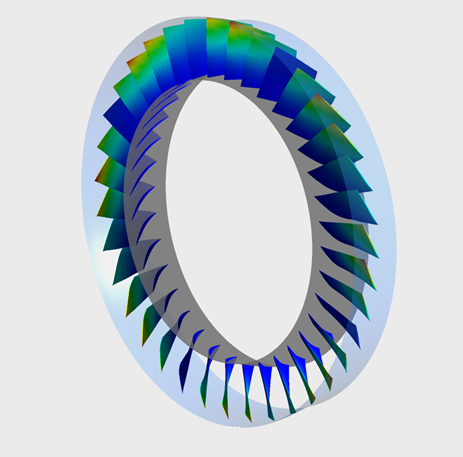
This tutorial uses an axial compressor to illustrate the basic concepts of setting up, running, and monitoring a transient blade row calculation with blade motion in CFX. The full geometry consists of one rotor containing 36 blades as seen in Figure 36.1: Single-row Reference Case Containing 36 Blades below.
For non-zero nodal diameters, there is a finite inter-blade phase angle (IBPA) between neighboring blades. This phase difference between the blades is defined as:

where
 is the number of blades and
 for an even number of blades and
 for an odd number of blades.
The following table compares the number of passages per component required to model a given nodal diameter when using periodic boundary conditions or the Fourier Transformation approach:
|
Nodal Diameter |
IBPA [deg] |
Number of Passages per Component to Model | |
|---|---|---|---|
|
Reference Case (Rotational Periodicity) |
Fourier Transformations | ||
|
0 |
0 |
1 |
2 |
|
1 |
10 |
36 |
2 |
|
2 |
20 |
18 |
2 |
|
3 |
30 |
12 |
2 |
|
4 |
40 |
9 |
2 |
|
5 |
50 |
36 |
2 |
|
6 |
60 |
6 |
2 |
|
7 |
70 |
36 |
2 |
|
8 |
80 |
9 |
2 |
|
9 |
90 |
4 |
2 |
For this tutorial, you will model a nodal diameter of four using the Fourier transformation approach with only two passages. The equivalent model using the periodic boundary conditions (reference case) requires nine passages, that is, a quarter of the original rotor.
The machine is rotating at 1800 [rad s^-1]. The inlet boundary condition is modeled as Total Pressure and Total Temperature in the stationary frame, with a specified flow direction in cylindrical components. The outlet boundary condition is set to an average static pressure of 138 [kPa], varying in the radial direction only. The inlet boundary profile is provided in a .csv file.
The blade vibration is modeled as forced periodic motion at a fixed frequency with a specified inter-blade phase angle. The frequency and displacement profile (mode shape) are obtained from cyclic symmetry calculations in Ansys Mechanical using a single blade model, and exported to a .csv file. For this case the vibration frequency is 1152.13 [Hz], and the maximum displacement for the mode shape is 0.00129 [m]. In order to use this single blade mode shape for multiple blade flow simulations, the profile must be replicated around the machine axis. This replicated profile contains a sector number identifying every copied section from the original profile. This sector number increases following the right hand rule around the machine axis. The sector number information can be used to determine the direction of the phase shift; that is, it can be used to determine whether the blade displacement is initiated on the blade with the higher or lower theta position.
The surface of revolution mesh motion boundary condition is used at the shroud to model the sliding of the mesh along the surface.
The vibration of the blades with IBPA results in a traveling wave pattern. For a model that has a rotating component:
A Forward Traveling Wave (FTW) is a wave traveling in the direction of machine rotation, and is associated with a positive IBPA value.
A Backward Traveling Wave (BTW) is a wave traveling in the direction opposite to machine rotation, and is associated with a negative IBPA value.
This tutorial models IBPA=+40°, which represents Nodal Diameter=4 for a forward traveling wave.
The hub surface nodes are set to be stationary. The shroud surface nodes are allowed to follow the blade displacement.
If this is the first tutorial you are working with, it is important to review the following topics before beginning:
Create a working directory.
Ansys CFX uses a working directory as the default location for loading and saving files for a particular session or project.
Download the
fourier_blade_flutter.zipfile here .Unzip
fourier_blade_flutter.zipto your working directory.Ensure that the following tutorial input files are in your working directory:
R37ATM_60k.gtmR37_inlet.csvR37_mode1_1p.csv
Set the working directory and start CFX-Pre.
For details, see Setting the Working Directory and Starting Ansys CFX in Stand-alone Mode.
This section describes the steady-state simulation setup for blade flutter in CFX-Pre and subsequent use of CFX-Solver Manager to obtain a solution. Although, the effect of mesh motion on a steady-state run is minimal, it will provide you with the initial conditions for the Fourier Transformation Blade Flutter case.
In CFX-Pre, select File > New Case.
Select General and click .
Select File > Save Case As.
Set File name to
FourierBladeFlutterIni.cfx.Click .
In the Outline tree view, right-click
Meshand select Import Mesh > CFX Mesh.The Import Mesh dialog box appears.
Configure the following setting(s):
Setting
Value
Filename
R37ATM_60k.gtm
Click Open.
This file contains a single passage mesh. The Fourier Transformation method requires two passages for any IBPA number.
In the Outline tree view, right-click Mesh >
R37ATM_60k.gtmand select Transform Mesh.The Mesh Transformation Editor dialog box appears.
Set Transformation to Turbo Rotation.
Configure the following setting(s):
Setting
Value
Rotation Option
Principal Axis
Axis
Z
Passages per Mesh
1
Passages to Model
2
Passages in 360
36
Click Apply and close the Mesh Transformation Editor dialog box.
The profile describing the frequency and blade mode shape for one blade is provided with this tutorial. In preparation for a two-passage Fourier Transformation setup, you will expand this profile and initialize it to be used for boundary condition specifications.
Select Tools > Edit Profile Data.
The Edit Profile Data dialog box appears.
Under Source Profile, click Browse
 .
.The Select Profile Data File dialog box appears.
From your working directory, select
R37_mode1_1p.csvand click Open.Set Write to Profile to
R37_mode1_36p.csv.Ensure that Initialize New Profile After Writing is selected so that the mode1 profile data will be automatically initialized using the expanded profile.
In the Transformations frame, click Add new item
 , set Name to
 Transformation 1, and click OK.Configure the following setting(s):
Setting
Value
Transformation 1
> Option
Expansion
Transformation 1
> Expansion Definition
> Rotation Option
Principal Axis
Transformation 1
> Expansion Definition
> Axis
Z
Transformation 1
> Expansion Definition
> Passages in Profile
1
Transformation 1
> Expansion Definition
> Passages in 360
36
Transformation 1
> Expansion Definition
> Expansion Option
Expand to Full Circle
Transformation 1
> Expansion Definition
> Theta Offset
0 [degree]
Click .
You have expanded the profile data coverage from one passage to 36
passages.
The expanded profile file is divided into sectors, as indicated by an extra data column named
Sector Tag. Sector 1 contains the original data, which covers one passage.
Sector 2 contains data for a second passage. The coordinates and displacement vector components
in sector 2 are rotated appropriately compared to the corresponding data in sector 1.
The inflow and mode1 functions are defined using profiles found
in the .csv files in your working directory.
You have already initialized the profile data for the mode1 functions (meshdisptot x(Initial X, Initial Y, Initial Z), meshdisptot y(Initial X, Initial Y, Initial Z), meshdisptot z(Initial X, Initial Y, Initial Z)) during the profile expansion process, due to use of the
Initialize New Profile After Writing option in the Edit Profile Data dialog box.
You will now initialize the profile data for the inflow functions (Total Pressure(r), Total Temperature(r), Velocity Axial(r), Velocity Circumferential(r), and Velocity Radial(r)):
Select Tools > Initialize Profile Data.
The Initialize Profile Data dialog box appears.
Beside Profile Data File, click Browse
.The Select Profile Data File dialog box appears.
From your working directory, select
R37_inlet.csv.Click Open.
Click .
The
inflowprofile data is read into memory.
Note: After profile data has been initialized from a file, the profile data file should not be deleted or otherwise removed from its directory. By default, the full file path to the profile data file is stored in CFX-Pre, and the profile data file is read directly by CFX-Solver each time the solver is started or restarted.
The fluid domain used for this simulation contains Air as an Ideal Gas. In addition to this, you will also set mesh motion for the blades.
Select Insert > Domain from the main menu.
The Insert Domain dialog box appears.
Set Name to
R1and click OK.Configure the following setting(s):
Tab
Setting
Value
Basic Settings
Location and Type
> Location
Entire Rotor Passage
Fluid and Particle Definitions...
> Fluid 1
> Material
Air Ideal Gas
Domain Models
> Pressure
> Reference Pressure
0 [atm]
Domain Models
> Domain Motion
> Option
Rotating
Domain Models
> Domain Motion
> Angular Velocity
-1800 [radian s^-1][ a ]
Domain Models
> Domain Motion
> Alternate Rotation Model
(Selected)
Domain Models
> Mesh Deformation
> Option
Regions of Motion Specified
Domain Models
> Mesh Deformation
> Displacement Rel. To
Initial Mesh
Domain Models
> Mesh Deformation
> Mesh Motion Model
> Option
Displacement Diffusion
Fluid Models
Heat Transfer
> Option
Total Energy
Turbulence
> Option
Shear Stress Transport
Turbulence
> Wall Function
Automatic
Turbulence
> Advanced Turbulence Control
> Reattachment Modification
(Selected)
Turbulence
> Advanced Turbulence Control
> Reattachment Modification
> Option
Reattachment Production
Click .
Create a new boundary named
R1 Inlet.Configure the following setting(s):
Tab
Setting
Value
Basic Settings
Boundary Type
Inlet
Location
Entire Rotor INFLOW
Frame Type
Stationary
Profile Boundary Conditions
> Use Profile Data
(Selected)
Profile Boundary Setup
> Profile Name
Inflow
Profile Boundary Setup
> Generate Values
(Click)
This causes profile values to be applied at the nodes on the inlet boundary. It also causes entries to be made in the Boundary Details tab. In order to later reset the velocity values at the inlet to match those that were originally read from the BC Profile file, revisit the Basic Settings tab for this boundary and click Generate Values.
Boundary Details
Mesh Motion
> Option
Stationary
Mass and Momentum
> Option
Stat. Frame Tot. Press.
Mass and Momentum
> Relative Pressure
Inflow.Total Pressure(r)[ a ]
Flow Direction
> Option
Cylindrical Components
Flow Direction
> Axial Component
Inflow.Velocity Axial(r)[ a ]
Flow Direction
> Radial Component
Inflow.Velocity Radial(r)[ a ]
Flow Direction
> Theta Component
Inflow.Velocity Circumferential(r)[ a ]
Turbulence
> Option
Medium (Intensity = 5%)
Heat Transfer
> Option
Stat. Frame Total Temp.
Heat Transfer
> Stat. Frame Tot. Temp.
Inflow.Total Temperature(r)[ a ]
Click .

Create a new boundary named
R1 Outlet.Configure the following setting(s):
Tab
Setting
Value
Basic Settings
Boundary Type
Outlet
Location
Entire Rotor OUTFLOW
Frame Type
Stationary
Boundary Details
Mesh Motion
> Option
Stationary
Mass and Momentum
> Option
Average Static Pressure
Mass and Momentum
> Relative Pressure
138 [kPa]
Mass and Momentum
> Pres. Profile Blend
1
Pressure Averaging
> Option
Radial Equilibrium
Pressure Averaging
> Radial Reference Position
> Option
Specified Radius
Pressure Averaging
> Radial Reference Position
> Specified Radius
0.215699 [m]
Click .
The hub, shroud and blade of the fluid region all require wall boundaries.
Create a new boundary named
R1 Hub.Configure the following setting(s):
Tab
Setting
Value
Basic Settings
Boundary Type
Wall
Location
Entire Rotor HUB
Frame Type
Rotating
Boundary Details
Mesh Motion
> Option
Stationary
Click .
Create a new boundary named
R1 Shroud.Configure the following setting(s):
Tab
Setting
Value
Basic Settings
Boundary Type
Wall
Location
Entire Rotor SHROUD
Frame Type
Rotating
Boundary Details
Mesh Motion
> Option
Surface of Revolution
Mesh Motion
> Axis Definition
> Option
Coordinate Axis
Mesh Motion
> Axis Definition
> Rotation Axis
Global Z
Mass and Momentum
> Wall Velocity
(Selected)
Mass and Momentum
> Wall Velocity
> Option
Counter Rotating Wall
Click .
Create a new boundary named
R1 Blade.Configure the following setting(s):
Tab
Setting
Value
Basic Settings
Boundary Type
Wall
Location
Entire Rotor BLADE
Frame Type
Rotating
Profile Boundary Conditions
> Use Profile Data
(Selected)
Profile Boundary Setup
> Profile Name
mode1
Boundary Details
Mesh Motion
> Option
Stationary
Click .
You will now create a pair of fluid-fluid domain interfaces along the tip gap for each blade.
Click Insert > Domain Interface and, in the dialog box that appears, set Name to
R1 Blade Tip
       Gap
and click OK.Configure the following setting(s):
Tab
Setting
Value
Basic Settings
Interface Type
Fluid Fluid
Interface Side 1
> Domain (Filter)
R1
Interface Side 1
> Region List
Rotor SHROUD TIP GGI SIDE 1
Interface Side 2
> Domain (Filter)
R1
Interface Side 2
> Region List
Rotor SHROUD TIP GGI SIDE 2
Interface Models
> Option
General Connection
Mesh Connection
Mesh Connection Method
> Mesh Connection
> Option
GGI
Click .
Click Insert > Domain Interface and, in the dialog box that appears, set Name to
R1 Blade Tip Gap
       2
and click OK.Configure the following setting(s):
Tab
Setting
Value
Basic Settings
Interface Type
Fluid Fluid
Interface Side 1
> Domain (Filter)
R1
Interface Side 1
> Region List
Rotor SHROUD TIP GGI SIDE 1 2
Interface Side 2
> Domain (Filter)
R1
Interface Side 2
> Region List
Rotor SHROUD TIP GGI SIDE 2 2
Interface Models
> Option
General Connection
Mesh Connection
Mesh Connection Method
> Mesh Connection
> Option
GGI
Click .
Click Insert > Domain Interface and, in the dialog box that appears, set Name to
R1 to R1
       Periodic
and click OK.Configure the following setting(s):
Tab
Setting
Value
Basic Settings
Interface Type
Fluid Fluid
Interface Side 1
> Domain (Filter)
R1
Interface Side 1
> Region List
Rotor PER1
Interface Side 2
> Domain (Filter)
R1
Interface Side 2
> Region List
Rotor PER2 2
Interface Models
> Option
Rotational Periodicity
Interface Models
> Axis Definition
> Option
Coordinate Axis
Interface Models
> Axis Definition
> Rotation Axis
Global Z
Mesh Connection
Mesh Connection Method
> Mesh Connection
> Option
GGI
Click .
In addition to the two fluid-fluid interfaces, the Fourier Transformation method requires a domain interface between the two passages. This interface method will be used by the Fourier Transformation method to collect information about the flow. The data will then be transferred back to the rotational periodic boundaries with the proper time lag.
Note: The periodic and sampling interfaces must use the GGI mesh connection.
Click Insert > Domain Interface and, in the dialog box that appears, set Name to
R1 Sampling
       Interface
and click OK.Configure the following setting(s):
Tab
Setting
Value
Basic Settings
Interface Type
Fluid Fluid
Interface Side 1
> Domain (Filter)
R1
Interface Side 1
> Region List
Rotor PER2
Interface Side 2
> Domain (Filter)
R1
Interface Side 2
> Region List
Rotor PER1 2
Interface Models
> Option
General Connection
Mesh Connection
Mesh Connection Method
> Mesh Connection
> Option
GGI
Click .
Fourier Transformation periodic boundary condition mappings
are affected by the mesh motion applied to the periodic interfaces.
You can prevent this by changing the mesh motion options for the Periodic and Sampling interfaces
to stationary.
In the Outline tree view, edit
Flow Analysis 1>R1>R1 to R1 Periodic Side 1.Configure the following setting(s):
Tab
Setting
Value
Boundary Details
Mesh Motion
> Option
Stationary
Click .
Repeat step 2 for
R1 to R1 Periodic Side 2,R1 Sampling Interface Side 1, andR1 Sampling Interface Side 2.
Click Write Solver Input File
 .
.Configure the following setting(s):
Setting
Value
File name
FourierBladeFlutterIni.def
Click .
Save the simulation.
From the Ansys CFX Launcher, start the CFX-Solver Manager. In CFX-Solver Manager:
Select File > Define Run
The Define Run dialog box is displayed.
Under Solver Input File, click Browse
and, in the dialog box that appears, select
FourierBladeFlutterIni.defand click Open.Select Double Precision.
Click Start Run.
CFX-Solver runs and attempts to obtain a solution. At the end of the run, a dialog box is displayed stating that the simulation has ended.
Ensure that Post-Process Results is cleared.
Click .
In this part of the tutorial, you will modify the steady-state simulation from the first part of the tutorial in order to add the transient blade flutter/moving mesh details and set up the case to use the Fourier Transformation method. The result from the steady-state simulation is used as an initial guess to speed up the convergence for the transient simulation.
This step involves opening the original simulation and saving it to a different location.
Ensure that the following tutorial input files are in your working directory:
FourierBladeFlutterIni.cfxFourierBladeFlutterIni_001.resR37_inlet.csvR37_mode1_36p.csv
Set the working directory and start CFX-Pre if it is not already running.
For details, see Setting the Working Directory and Starting Ansys CFX in Stand-alone Mode.
If the original simulation is not already opened, then open
FourierBladeFlutterIni.cfx.Save the case as
FourierBladeFlutterTime.cfxin your working directory.
Modify the analysis type as follows:
Edit
Analysis Type.Configure the following setting(s):
Setting
Value
Analysis Type
> Option
Transient Blade Row
Click .
Modify the domain as follows:
In the Outline tree view, edit
Flow Analysis 1>R1.Configure the following setting(s):
Tab
Setting
Value
Basic Settings
Domain Models
> Passage Definition
> Pass. in Component
2
Domain Models
> Passage Definition
> Passages in 360
36
Click .
Next, you will create expressions defining the frequency, maximum periodic displacement and scaling factor that will be used in the blade boundary definition.
From the main menu, select Insert > Expressions, Functions and Variables > Expression.
In the Insert Expression dialog box, type
VibrationFrequency.Click .
Set Definition to
1152.13 [Hz].Click Apply to create the expression.
You will create an expression defining the maximum periodic displacement.
Create an expression called
MaxPeriodicDisplacement.Set Definition to
0.0015 [m].Click Apply.
You will use the maximum periodic displacement from above to calculate the scaling factor. The scaling factor is chosen as the maximum amplitude the blade will deform, normalized by the maximum amplitude of the mode shape provided. The maximum amplitude for the blade is set to approximately 2% of the maximum span of the blade.
Create an expression called
ScalingFactor.Set Definition to
MaxPeriodicDisplacement/0.00129[m].Click Apply.
In the Outline tree view, edit
Flow Analysis 1>R1>R1 Blade.Configure the following setting(s):
Tab
Setting
Value
Basic Settings
Boundary Type
Wall
Location
Entire Rotor BLADE
Frame Type
Rotating
Profile Boundary Conditions
> Use Profile Data
(Selected)
Profile Boundary Setup
> Profile Name
mode1
Profile Boundary Setup
> Generate Values
(Click)
This sets the options under the Boundary Details tab.
Boundary Details
Mesh Motion
> Option
Periodic Displacement
Mesh Motion
> Periodic Displacement
> Option
Cartesian Components
Mesh Motion
> Periodic Displacement
> X Component
mode1.meshdisptot x(Initial X,Initial Y,Initial Z)
Mesh Motion
> Periodic Displacement
> Y Component
mode1.meshdisptot y(Initial X,Initial Y,Initial Z)
Mesh Motion
> Periodic Displacement
> Z Component
mode1.meshdisptot z(Initial X,Initial Y,Initial Z)
Mesh Motion
> Periodic Displacement
> Frequency
mode1.Frequency()
Mesh Motion
> Periodic Displacement
> Scaling
ScalingFactor[ a ]
Mesh Motion
> Periodic Displacement
> Phase Angle
> Option
Nodal Diameter (Phase Angle Multiplier)
Mesh Motion
> Periodic Displacement
> Phase Angle
> Nodal Diameter Mag.
4
Mesh Motion
> Periodic Displacement
> Phase Angle
> Traveling Wave Dir.
Forward
Mesh Motion
> Periodic Displacement
> Phase Angle
> Passage Number
mode1.Sector Tag(Initial X,Initial Y,Initial Z)
Click .
In this section, you will set the simulation to be solved using the Fourier Transformation method.
In the Outline tree view, edit
Flow Analysis 1>Transient Blade Row Models.Configure the following setting(s):
Setting
Value
Transient Blade Row Model
> Option
Fourier Transformation
Under Fourier Transformation, click Add new item
, accept the default name, and click OK.Configure the following setting(s):
Setting
Value
Fourier Transformation
> Fourier Transformation 1
> Option
Blade Flutter
Fourier Transformation
> Fourier Transformation 1
> Phase Corrected Intf.
R1 to R1 Periodic
Fourier Transformation
> Fourier Transformation 1
> Sampling Dom. Intf.
R1 Sampling Interface
Fourier Transformation
> Fourier Transformation 1
> Blade Boundary
R1 Blade
Transient Method
> Option
Time Integration
Transient Method
> Time Period
> Option
Value
Transient Method
> Time Period
> Period
1/VibrationFrequency[ a ]
Transient Method
> Time Steps
> Option
Number of Timesteps per Period
Transient Method
> Time Steps
> Timesteps/Period
72[ b ]
Transient Method
> Time Duration
> Option
Number of Periods per Run
Transient Method
> Time Duration
> Periods per Run
10
Click .
In this section you will create monitor points to monitor flow properties, integrated flow quantities, and mesh displacement. Monitor points provide useful information on the quality of the reference phase and frequency produced by the simulation. These monitor points should also be used to monitor convergence and patterns during the simulation.
Note:
When comparing your Fourier Transformation plots to those from the reference case, make sure the monitor points are placed in the same relative locations with respect to the initial configuration in both cases.
Monitoring pressure and velocity provides feedback on the momentum equations, while monitoring temperature provides feedback on the energy equations. Monitor points help check that the solver equations are being solved correctly.
Set up the solver to output transient results files. The transient blade row analysis type offers the Fourier compression method of storing transient periodic data.
Click Output Control
 .
.Click the Trn Results tab.
Configure the following setting(s):
Setting
Value
Transient Blade Row Results
> Extra Output Variables List
(Selected)
Transient Blade Row Results
> Extra Output Variables List
> Extra Output Var. List
Total Pressure, Total Temperature, Total Mesh Displacement, Wall Work Density, Wall Power Density[ a ]
Click .
Click the Monitor tab.
Select Monitor Objects.
Add an Efficiency Output monitor:
Setting
Value
Monitor Objects
> Efficiency Output
(Selected)
Monitor Objects
> Efficiency Output
> Option
Output to Solver Monitor
Monitor Objects
> Efficiency Output
> Inflow Boundary
R1 Inlet
Monitor Objects
> Efficiency Output
> Outflow Boundary
R1 Outlet
Monitor Objects
> Efficiency Output
> Efficiency Type
Compression
Monitor Objects
> Efficiency Output
> Value
Total to Total
You will set up three types of monitors for this simulation. Firstly, you will create a set of monitor points to monitor variables at specific cylindrical coordinates within the domain. Cylindrical coordinates are useful in turbomachinery applications because they allow you to place monitor points with the same relative position inside different passages by shifting the theta component by the equivalent passage pitch. Next, you will create a second set of monitors to monitor the values of expressions. Finally, you will create a third set of monitors to monitor aerodynamic damping.
Create monitor points by configuring the following settings:
Setting
Value
Monitor Objects
> Monitor Points and Expressions
Create a monitor point named
LE1pass1[ a ]Monitor Objects
> Monitor Points and Expressions
> LE1pass1
> Option
Cylindrical Coordinates
Monitor Objects
> Monitor Points and Expressions
> LE1pass1
> Output Variables List
Pressure, Temperature, Total Pressure, Total Temperature, Velocity, Velocity in Stn Frame[ b ]
Monitor Objects
> Monitor Points and Expressions
> LE1pass1
> Position Axial Comp.
0 [m]
Monitor Objects
> Monitor Points and Expressions
> LE1pass1
> Position Radial Comp.
0.23 [m]
Monitor Objects
> Monitor Points and Expressions
> LE1pass1
> Position Theta Comp.
-7.5 [degree]
Click .
Create additional monitor points with the same output variables. The names and cylindrical coordinates are listed below:
Name
Coordinates
LE1pass2
(0 [m], 0.23 [m], 2.5 [degree])
LE2pass1
(0 [m], 0.23 [m], -2.5 [degree])
LE2pass2
(0 [m], 0.23 [m], 7.5 [degree])
TE1pass1
(0.05 [m], 0.23 [m], 0 [degree])
TE1pass2
(0.05 [m], 0.23 [m], 10 [degree])
TE2pass1
(0.05 [m], 0.23 [m], 5 [degree])
TE2pass2
(0.05 [m], 0.23 [m], 15 [degree])
Create additional monitor points with the following expressions:
Name
Expression
Force on Blade
force()@REGION:Rotor BLADE
Force on Blade 2
force()@REGION:Rotor BLADE 2
Max Displ Blade
maxVal(Total Mesh Displacement)@REGION:Rotor BLADE
Max Displ Blade 2
maxVal(Total Mesh Displacement)@REGION:Rotor BLADE 2
Power on Blade
areaInt(Wall Power Density)@REGION:Rotor BLADE
Power on Blade 2
areaInt(Wall Power Density)@REGION:Rotor BLADE 2
Work on Blade
areaInt(Wall Work Density)@REGION:Rotor BLADE
Work on Blade 2
areaInt(Wall Work Density)@REGION:Rotor BLADE 2
Create aerodynamic damping monitors by configuring the following settings:
Setting
Value
Monitor Objects
> Aerodynamic Damping
Create an aerodynamic damping object named
Aerodynamic Damping 1.Monitor Objects
> Aerodynamic Damping
> Aerodynamic Damping 1
> Option
Full Period Integration
Monitor Objects
> Aerodynamic Damping
> Aerodynamic Damping 1
> Location Type
> Option
Mesh Regions
Monitor Objects
> Aerodynamic Damping
> Aerodynamic Damping 1
> Location Type
> Location
Rotor BLADE
Monitor Objects
> Aerodynamic Damping
Create an aerodynamic damping object named
Aerodynamic Damping 2.Monitor Objects
> Aerodynamic Damping
> Aerodynamic Damping 2
> Option
Full Period Integration
Monitor Objects
> Aerodynamic Damping
> Aerodynamic Damping 2
> Location Type
> Option
Mesh Regions
Monitor Objects
> Aerodynamic Damping
> Aerodynamic Damping 2
> Location Type
> Location
Rotor BLADE 2
Monitor Objects
> Aerodynamic Damping
Create an aerodynamic damping object named
Aerodynamic Damping 3.Monitor Objects
> Aerodynamic Damping
> Aerodynamic Damping 3
> Option
Moving Integration Interval
Monitor Objects
> Aerodynamic Damping
> Aerodynamic Damping 3
> Location Type
> Option
Mesh Regions
Monitor Objects
> Aerodynamic Damping
> Aerodynamic Damping 3
> Location Type
> Location
Rotor BLADE
Click OK.

Click Write Solver Input File
.Configure the following setting(s):
Setting
Value
File name
FourierBladeFlutterTime.def
Click .
If a Physics Validation Summary message appears, indicating one global warning, click to continue. The warning is about initial values, which will be supplied at run-time.
Save the case.
To reduce the simulation time for the blade flutter case, the simulation will be initialized using the steady-state case.
In CFX-Solver Manager:
Click File > Define Run.
Under Solver Input File, click Browse
and select FourierBladeFlutterTime.def.Select Double Precision.
On the Initial Values tab, select Initial Values Specification.
Under Initial Values Specification > Initial Values, select
Initial Values 1.Under Initial Values Specification > Initial Values > Initial Values 1 Settings > File Name, click Browse
.Select
FourierBladeFlutterIni_001.resfrom your working directory.Click Open.
Set Initial Values Specification > Use Mesh From, to
Solver Input File.Click .
CFX-Solver runs and attempts to obtain a solution. This can take a long time depending on your system. Eventually a dialog box is displayed.
Before the simulation begins, the "Transient Blade Row Post-processing Information" summary in the CFX-Solver Output file will display the time step range over which the solver will accumulate the Fourier coefficients. A "Fourier Transformation Stability" summary appears in the CFX-Solver Output file, as well as the time step at which the full Fourier Transformation model is activated.
When CFX-Solver is finished, you can optionally skip to Postprocessing the Blade Flutter Solution.
In this part of the tutorial, you will modify the Time Integration solution method case that was set up in the previous part of the tutorial in order to use the Harmonic Balance solution method. As in the previous part, the result from the steady-state simulation is used as an initial guess to speed convergence.
This step involves opening the Time Integration simulation and saving it to a different location.
Ensure that the following tutorial input files are in your working directory:
FourierBladeFlutterTime.cfxFourierBladeFlutterIni_001.resR37_inlet.csvR37_mode1_36p.csv
Set the working directory and start CFX-Pre if it is not already running.
For details, see Setting the Working Directory and Starting Ansys CFX in Stand-alone Mode.
If the Time Integration simulation is not already opened, then open
FourierBladeFlutterTime.cfx.Save the case as
FourierBladeFlutterHarmonic.cfxin your working directory.
There are many common steps between setting up Time Integration and Harmonic Balance Flutter cases, including using the same Fourier Transformation pitch change model. Here, only the differences are highlighted.
In this section, you will change the transient method to Harmonic
Balance.
In the Outline tree view, edit
Flow Analysis 1>Transient Blade Row Models.Configure the following setting(s):
Tab
Setting
Value
Basic Settings
Transient Method
> Option
Harmonic
    Balance
Transient Method
> Number of Modes
3
Note that, in the Transient Blade Row Models details view, on the Basic Settings tab, the settings for Time Period, Time Steps and Time Duration have disappeared.
Click OK.
Most blade flutter cases require only one mode. However, if the flow contains discontinuities like shocks that happen to oscillate with the vibration, then retaining 3 modes will be necessary for an accurate solution.
There is no need to specify the period involved when selecting Harmonic Balance in combination with the Fourier Transformation model. It will be obtained from the usual location for a blade flutter run (that is, in the Mesh Motion settings for the vibrating blade).
Click Solver Control
 .
.Configure the following setting(s):
Tab
Setting
Value
Basic Settings
Transient Scheme
> Option
Harmonic Balance
Convergence Control
> Min. Iterations
1
Convergence Control
> Max. Iterations
200
Convergence Control
> Fluid Timescale Control
> Timescale Control
Physical Timescale
Convergence Control
> Fluid Timescale Control
> Physical Timescale
1/(15*VibrationFrequency)
Convergence Criteria
> Residual Type
RMS
Convergence Criteria
> Residual Target
1e-5
Click OK.
The time periods involved in this case are:
The blade vibrating period
The period defined by the rotating domain
The physical timescale is usually set as a fraction of the smallest time period involved. In this case, the blade vibrating period is the smallest time period involved, and 1/15th of that period is used as the physical timescale. A larger physical timescale speeds convergence but can lower stability. In general, if the solution becomes unstable or does not converge, you should use a smaller fraction when computing the physical timescale.
In this section you will create monitor points to monitor flow properties, integrated flow quantities, and mesh displacement. Monitor points provide useful information on the quality of the reference phase and frequency produced by the simulation. These monitor points should also be used to monitor convergence and patterns during the simulation.
Note:
When comparing your Fourier Transformation plots to those from the reference case, make sure the monitor points are placed in the same relative locations with respect to the initial configuration in both cases.
Monitoring pressure and velocity provides feedback on the momentum equations, while monitoring temperature provides feedback on the energy equations. Monitor points help check that the solver equations are being solved correctly.
Set up the solver to output transient results files. The transient blade row analysis type offers the Fourier compression method of storing transient periodic data.
Click Output Control
.Click the Trn Results tab.
Configure the following setting(s):
Setting
Value
Transient Blade Row Results
> Extra Output Variables List
(Selected)
Transient Blade Row Results
> Extra Output Variables List
> Extra Output Var. List
Total Pressure, Total Temperature, Total Mesh Displacement, Wall Work Density, Wall Power Density[ a ]
Click .
Click the Monitor tab.
You have already set up monitors for variables, values of expressions, and aerodynamic damping. The aerodynamic damping monitors need to be modified.
Modify the aerodynamic damping monitors by configuring the following settings:
Setting
Value
Monitor Objects
> Aerodynamic Damping
Select the aerodynamic damping object named
Aerodynamic Damping 1.Monitor Objects
> Aerodynamic Damping
> Aerodynamic Damping 1
> Option
Fourier Integration
Monitor Objects
> Aerodynamic Damping
> Aerodynamic Damping 1
> Location Type
> Option
Mesh Regions
Monitor Objects
> Aerodynamic Damping
> Aerodynamic Damping 1
> Location Type
> Location
Rotor BLADE
Monitor Objects
> Aerodynamic Damping
Select the aerodynamic damping object named
Aerodynamic Damping 2.Monitor Objects
> Aerodynamic Damping
> Aerodynamic Damping 2
> Option
Fourier Integration
Monitor Objects
> Aerodynamic Damping
> Aerodynamic Damping 2
> Location Type
> Option
Mesh Regions
Monitor Objects
> Aerodynamic Damping
> Aerodynamic Damping 2
> Location Type
> Location
Rotor BLADE 2
Monitor Objects
> Aerodynamic Damping
Delete the aerodynamic damping object named
Aerodynamic Damping 3.(Note that this object is a copy of
Aerodynamic Damping 1.)Click .
Click Write Solver Input File
.Configure the following setting(s):
Setting
Value
File name
FourierBladeFlutterHarmonic.def
Click .
Save the case.
To reduce the simulation time for the blade flutter case, the simulation will be initialized using the steady-state case.
In CFX-Solver Manager:
Click File > Define Run.
Under Solver Input File, click Browse
and select FourierBladeFlutterHarmonic.def.Select Double Precision.
On the Initial Values tab, select Initial Values Specification.
Under Initial Values Specification > Initial Values, select
Initial Values 1.Under Initial Values Specification > Initial Values > Initial Values 1 Settings > File Name, click Browse
.Select
FourierBladeFlutterIni_001.resfrom your working directory.Click Open.
Set Initial Values Specification > Use Mesh From, to
Solver Input File.Click .
CFX-Solver runs and attempts to obtain a solution. This can take a long time depending on your system. Eventually a dialog box is displayed.
The postprocessing steps outlined here can be equally used on either of the Blade Flutter solutions obtained in Defining and Obtaining a Solution for the Time Integration Solution Method Case and Defining and Obtaining a Solution for the Harmonic Balance Solution Method Case. The results should be similar and the differences between the two will be minimized by comparing a time-resolved transient case to a modal-resolved harmonic balance case (that is, a case where increasing the number of modes or time planes does not result in solution change).
Some of the monitor points of the Time Integration case show instantaneous values that oscillate about certain values. The corresponding monitor points of the Harmonic Balance case show values that are time-averaged over the vibration period.
Select Workspace > New Monitor and accept the default name.
Under the Plot Lines tab, expand the USER POINT branch and select
Work on Blade.Click Apply.
On the Range Settings tab, set Plot Data By to
Simulation Time.This displays a simulation time history of the work on blade 1.
Click the Aerodynamic Damping tab.
Observe the aerodynamic damping monitors. The monitor values represent mechanical work done by the blade on the fluid over the last period of mesh motion. If the monitor values remain positive (after the case has converged), then the vibration is damped (for the frequency being studied).
Click the Efficiency tab.
Observe the monitor points related to efficiency.
When done with the CFX-Solver Manager, you can continue examining the solutions with CFD-Post.
A transient blade row analysis calculation creates a number of solution variables in addition to those added in Setting Output Control and Creating Monitor Points. These variables are compressed using a discrete Fourier Transformation and the corresponding coefficients are stored in the results file. CFD-Post can expand this transformation for the variable of interest at any given time value. The time step selector shows time values that are representative of the values used by the solver. In addition to the existing time values, additional time values can be added or removed as deemed necessary.
In this section, you will create a few plots to illustrate the use of the time step selector for a transient blade row analysis. You will also create a user defined variable for the total wall work, and use that variable to create a contour and an animation of the blade.
Note: When CFD-Post starts, you may see a message regarding transient blade row postprocessing. If you do, click .
In CFD-Post, with results loaded:
Select Insert > Variable and set the name to
Total Wall Work.Configure the following setting(s):
Name
Setting
Value
Total Wall Work
Method
Expression
Scalar
(Selected)
Expression
Wall Work Density * Area
Calculate Global Range
(Selected)
Click Apply to create the new variable.
You can review the new
Total Wall Workvariable on the Variables tab, under theUser Definedbranch.
Click Insert > Contour and accept the default name.
Configure the following setting(s):
Tab
Setting
Value
Geometry
Locations
R1 Blade
Variable
Total Wall Work
Range
Local
# of Contours
21
Render
Show Contour Lines
(Selected)
Constant Coloring
(Selected)
Color Mode
Default
Click Apply.
The contour plot shows instantaneous values for Total
Wall Work.
Using the contour plot created above, you will now create an
animation of the Total Wall Work on the blade
for the first phase.
Click Timestep Selector
 .
.The Timestep Selector dialog box appears.
Set Timestep Sampling to
Uniform.Select the time value of
0 [s].Click Apply.
Select Tools > Animation or click Animation
 .
.The Animation dialog box appears.
Set Type to Timestep Animation.
Ensure that Control By is set to
Timestep.Select Specify Range for Animation.
Set Start Timestep to
0and End Timestep to10.Select Save Movie.
Set Format to
MPEG1.Click Browse
next
to Save Movie to set a path and filename for
the movie file.If the file path is not given, the file will be saved in the directory from which CFD-Post was launched.
Click .
The movie filename (including path) is set, but the movie is not yet created.
If Current Timestep is not
0(shown in the Animation dialog box), click To First Timestep to load it.
 Wait for CFD-Post to finish loading the objects for this frame before proceeding.
Click Play the animation
 .
.The movie will be created as the animation proceeds. This will be slow, since a time step must be loaded and objects must be created for each frame. To view the movie file, you need to use a viewer that supports the MPEG format.
When you have finished, close CFD-Post.