


CFD simulations based on RANS models are typically carried out in 'steady-state' model (see Section 3.2). In most cases the following settings are appropriate:
Coupled solver
Pseudo-transient
Use default proposed time step
In case of convergence problems vary time step
Second order momentum
Second order turbulence
This is very helpful for unstructured grids and or grids not well aligned with the flow. For hexahedral grids with good flow alignment the difference between 1st and 2nd order space discretization is typically moderate.
Experience has shown that 2nd order space discretization for turbulence does not have an overall negative influence on convergence – it is therefore recommended.
The following topics are discussed:
A drastic example for the danger of non-converged solutions is the following flow around a
generic airplane geometry with high-lift devices (slats upstream and flaps downstream of the
wing employed) deployed. The simulations for the JAXA geometry were carried out in the framework
of the 3rd AIAA CFD High Lift prediction Workshop
(https://hiliftpw.larc.nasa.gov/Workshop3/geometries.html). A first simulation with the SST
model using default model and steady state settings resulted in a substantial under-prediction
of the maximum lift coefficient ( ) due to a massive separation on the main wing. This can be seen in Figure 12.159: Figure 96: Wall shear stress for high-lift airplane simulation for
  =18 . Left: Simulation in 'steady-state mode'. Right: Simulation in 'unsteady mode'. (left) showing the skin friction on the surface for the
'steady-state' set-up for an angle of attack of
=18 . Left: Simulation in 'steady-state mode'. Right: Simulation in 'unsteady mode'. (left) showing the skin friction on the surface for the
'steady-state' set-up for an angle of attack of  . At first, this was attributed to the SST model's separation prediction
capabilities, which were apparently interpreted as being overly 'aggressive' for this case. For
this reason, the
. At first, this was attributed to the SST model's separation prediction
capabilities, which were apparently interpreted as being overly 'aggressive' for this case. For
this reason, the  coefficient in the SST model was increased to
  1 to reduce separation sensitivity. However, it was found that convergence for
the case with the default SST model setting was poor and the case was therefore re-run with
unsteady solver settings. The difference due to this change in numerical settings was dramatic
as shown in Figure Figure 96 (right) which shows the skin friction distribution for the unsteady
run. The unsteady set-up allowed the simulation to 'escape' from the incorrect flow topology and
move to a more realistic and much less separated condition.
1 to reduce separation sensitivity. However, it was found that convergence for
the case with the default SST model setting was poor and the case was therefore re-run with
unsteady solver settings. The difference due to this change in numerical settings was dramatic
as shown in Figure Figure 96 (right) which shows the skin friction distribution for the unsteady
run. The unsteady set-up allowed the simulation to 'escape' from the incorrect flow topology and
move to a more realistic and much less separated condition.
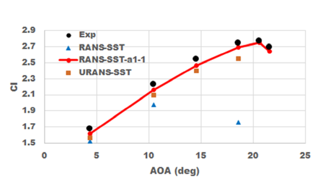
The effect on the lift coefficient can be seen in Figure 12.160: Lift coefficient, CI, for high-lift aircraft simulation versus angle of attack (AOA). RANS-SST with default and 'steady state mode', SST with a1=1.0 and 'steady state mode' and URANS-SST with default SST and 'unsteady mode' set-up. which
contains three curves. One for SST-default and 'steady state mode' one for SST with
 (instead of default
  ) and again 'steady state mode' and finally with SST default (
 ) and 'unsteady mode'. The change in the a1 coefficient results in less
separation and therefore a better agreement with the exp. data. However, such a change in
) and 'unsteady mode'. The change in the a1 coefficient results in less
separation and therefore a better agreement with the exp. data. However, such a change in
 is not justified from a physics standpoint, when considering at 2D airfoil
performance (see 4.2.2). Alternatively, the solution was also improved significantly by just
switching from the steady-state set-up to the unsteady set-up. The lift for the URANS simulation
is still somewhat lower than the experiment, but by a much lower factor compared to the steady
run. There is also indication that including laminar-turbulent transition in the simulation will
further increase the lift curve, so that the remaining difference can partly be attributed to
this effect. Besides such details, the important message here is that the difference between the
steady and unsteady solutions with identical turbulence model settings can be larger than the
differences between strongly different turbulence model settings.
is not justified from a physics standpoint, when considering at 2D airfoil
performance (see 4.2.2). Alternatively, the solution was also improved significantly by just
switching from the steady-state set-up to the unsteady set-up. The lift for the URANS simulation
is still somewhat lower than the experiment, but by a much lower factor compared to the steady
run. There is also indication that including laminar-turbulent transition in the simulation will
further increase the lift curve, so that the remaining difference can partly be attributed to
this effect. Besides such details, the important message here is that the difference between the
steady and unsteady solutions with identical turbulence model settings can be larger than the
differences between strongly different turbulence model settings.
Figure 12.159: Figure 96: Wall shear stress for high-lift airplane simulation for =18 . Left: Simulation in 'steady-state mode'. Right: Simulation in 'unsteady mode'.
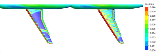
Figure 12.160: Lift coefficient, CI, for high-lift aircraft simulation versus angle of attack (AOA). RANS-SST with default and 'steady state mode', SST with a1=1.0 and 'steady state mode' and URANS-SST with default SST and 'unsteady mode' set-up.
It is important to stress that situations like the one shown above appear very seldomly, but they can happen in CFD. The exact cause for such scenarios is not easy to determine. However, there are some contributing factors:
Large variation in size of geometric features (in this case the thin pylons holding the slat vs the size of the airfoil).
Large variation in cell size between different regions (often because of the first bullet).
Large aspect ratio grids in the domain.
Potential for topology changes in the flowfield – meaning that the flow can change from 'attached' to stalled' on certain sections of the wing.
Local regions of unsteady flow with relevance to the overall flow topology.