| Applicable Products: | Ansys Multiphysics, Ansys Mechanical, Ansys Structural |
| Level of Difficulty: | Easy |
| Interactive Time Required: | 60 to 90 minutes |
| Discipline: | Structural |
| Analysis Type: | Linear static |
| Element Types Used: | PLANE183 |
| Features Demonstrated: | Solid modeling including primitives, Boolean operations, and fillets; tapered pressure load; deformed shape and stress displays; listing of reaction forces; examination of structural energy error |
| Help Resources: | Structural Static Analysis and PLANE183 |
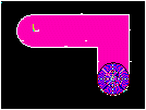
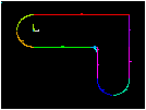
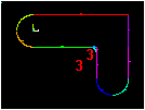
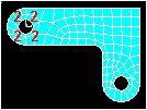
This is a simple, single-load-step, structural static analysis of a corner angle bracket. The upper-left pin hole is constrained (welded) around its entire circumference, and a tapered pressure load is applied to the bottom of the lower-right pin hole. The US Customary system of units is used.
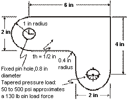
Objective: Demonstrate a typical Mechanical APDL analysis procedure.
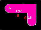
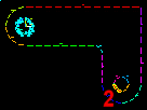
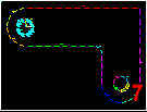
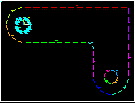
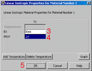
The dimensions of the corner bracket are shown in the accompanying figure. The bracket is made of A36 steel with a Young’s modulus of 30E6 psi and Poisson’s ratio of .27.
Because the bracket is thin in the z direction (1/2 inch thickness) compared to its x and y dimensions, and because the pressure load acts only in the x-y plane, assume plane stress for the analysis.
Your approach is to use solid modeling to generate the 2D model and automatically mesh it with nodes and elements. (An alternative approach is to create the nodes and elements directly.)
Use the information in the problem description and the steps below as a guideline in solving the problem on your own. Or, use the detailed interactive step-by-step solution by selecting the link for step 1.
Build Geometry
2. Change plot controls and replot.
3. Change working plane to polar and create first circle.
4. Move working plane and create second circle.
5. Add areas.
10. Move working plane and create second pin hole.
11. Subtract pin holes from bracket.
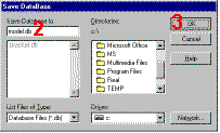
12. Save the database as model.db.
Define Materials
13. Set Preferences.
14. Define Material Properties.
15. Define element types and options.
Generate Mesh
17. Mesh the area.
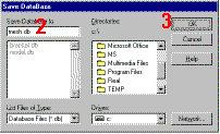
18. Save the database as mesh.db.
Apply Loads
19. Apply displacement constraints.
Obtain Solution
21. Solve.
Review Results
22. Enter the general postprocessor and read in the results.
24. Plot the von Mises equivalent stress.
This is the beginning of preprocessing.
There are several ways to create the model geometry within Mechanical APDL, some more convenient than others. The first step is to recognize that you can construct the bracket easily with combinations of rectangles and circle Primitives.
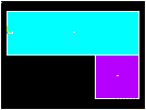
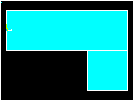
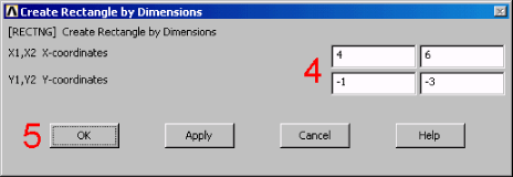
Select an arbitrary global origin location, then define the rectangle and circle primitives relative to that origin. For this analysis, use the center of the upper-left hole. Begin by defining a rectangle relative to that location.
 |
  |
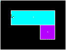
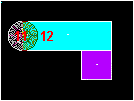
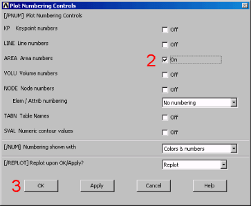
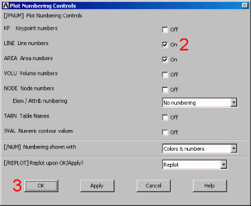
The area plot shows both rectangles, which are areas, in the same color. To more clearly distinguish between areas, turn on area numbers and colors. The "Plot Numbering Controls" dialog box on the Utility Menu controls how items are displayed in the Graphics Window. By default, the program performs a replot upon execution of the dialog box. The replot operation repeats the last plotting operation that occurred (in this case, an area plot).
|
 |
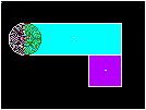
Create the half circle at each end of the bracket. You will actually create a full circle on each end and then combine the circles and rectangles with a Boolean add operation (discussed in step 5). To create the circles, you will use and display the working plane (WP).
Before you begin, use the Pan-Zoom-Rotate graphics-control tool to zoom out within the Graphics Window to see more of the circles as you create them.
|
   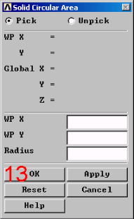 |
While positioning the cursor for picking, the dynamic WP X and Y values are displayed in the Solid Circular Area dialog.
As an alternative to picking, you can type the values along with the radius into the appropriate fields.
To create the circle at the other end of the bracket in the same way, first move the working plane to the origin of the circle. The simplest way to do so without entering number offsets is to move the WP to an average keypoint location by picking the keypoints at the bottom corners of the lower-right rectangle.
Pick keypoint at lower left corner of rectangle.
Pick keypoint at lower right of rectangle.
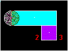
OK to close picking menu.

Pick center point at:
WP X = 0
WP Y = 0
Move mouse to radius of 1 and click left button to create circle.
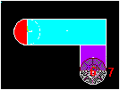
OK to close picking menu.
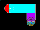
Toolbar: SAVE_DB.
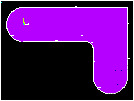
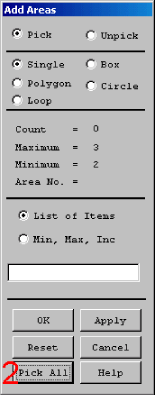
Now that the appropriate pieces of the model (rectangles and circles) are defined, add them together so the model becomes one continuous piece. Use the Boolean add operation for areas.
|
 |
|
|
|
  |
(toggle on)
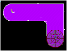
Pick center point at:
WP X = 0 (in Graphics Window)
WP Y = 0
Move mouse to radius of .4 (shown in the picking menu) and click left button to create circle.
OK to close picking menu.
Pick center point at:
WP X = 0 (in Graphics Window)
WP Y = 0
Move mouse to radius of .4 (shown in the picking menu) and click left mouse button to create circle.
OK to close picking menu.
(toggle off)
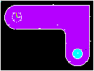
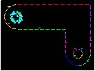
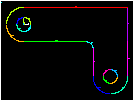
It appears that one of the pin-hole areas is missing; however, it is there (indicated by the presence of its lines). You cannot see it in the final display because the bracket area is drawn on top of it. An easy way to see all areas is to plot the lines instead.
Toolbar: SAVE_DB.
Pick bracket as base area from which to subtract.
Apply (in picking menu).
Pick both pin holes as areas to be subtracted.
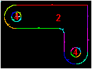
OK to subtract holes and close picking menu.

In preparation for defining materials, set preferences so that only materials pertaining to a structural analysis are available.
(check) "Individual discipline(s) to show in the GUI" = Structural
[OK] to apply filtering and close the dialog box.
To define material properties, there is only one material for the bracket, A36 Steel, with given values for Young’s modulus of elasticity and Poisson’s ratio.
|
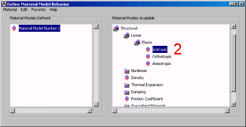  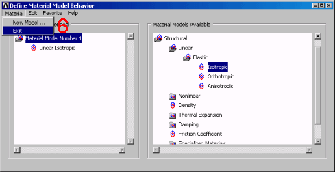 |
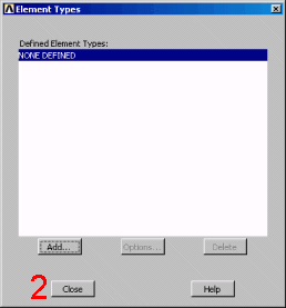
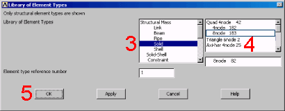
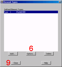
In any analysis, you select elements from a library of element types and define the appropriate ones for the analysis. In this case, only one element type is used: PLANE183, a 2D, quadratic, structural, higher-order element.
A higher-order element enables you to have a coarser mesh than with lower-order elements while still maintaining solution accuracy. Also, Mechanical APDL generates some triangle-shaped elements in the mesh that would otherwise be inaccurate when using used lower-order elements.
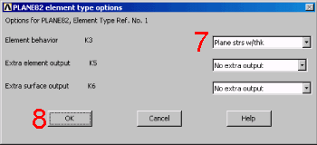
Specify plane stress with thickness as an option for PLANE183. (Thickness is defined as a real constant in Step 16: Define real constants..)
|
    |
Assuming plane stress with thickness, enter the thickness as a real constant for PLANE183:
Add a real constant set.
OK for PLANE183.
Enter .5 for THK.
OK to define the real constant and close the dialog box.
Close the real constant dialog box.
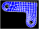
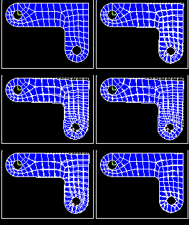
You can mesh the model without specifying mesh-size controls. If you are unsure of how to determine mesh density, you can allow Mechanical APDL to apply a default mesh. For this model, however, you will specify a global element size to control overall mesh density.
 |
  |
Your mesh may vary slightly from the mesh shown. You may see slightly different results during postprocessing. For a discussion of results accuracy, see Planning Your Approach.
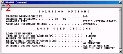
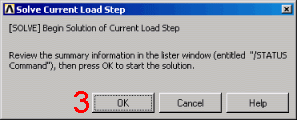
This step represents the beginning of the solution phase.
A new, static analysis is the default, so specifying an analysis type for this problem is unnecessary. Also, no analysis options exist for this problem.
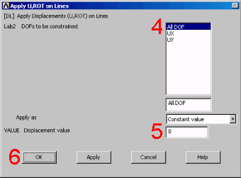
You can apply displacement constraints directly to lines.
|
 |
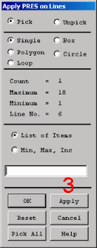
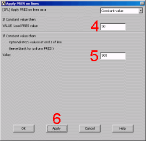
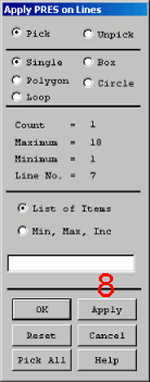
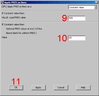
Apply the tapered pressure load to the bottom-right pin hole. (Tapered here means varying linearly.)
When a circle is created in Mechanical APDL, four lines define the perimeter; therefore, apply the pressure to two lines making up the lower half of the circle. Because the pressure tapers from a maximum value (500 psi) at the bottom of the circle to a minimum value (50 psi) at the sides, apply pressure in two separate steps, with reverse tapering values for each line.
The Mechanical APDL convention for pressure loading is that a positive load value represents pressure into the surface (compressive).
|
    |
|

|
Mechanical APDL stores the results of this single-load-step problem in the database and in the results file, Jobname.RST (or Jobname.RTH for thermal, Jobname.RMG for magnetic). The database can contain only one set of results at any given time, so in a multiple-load-step or multiple-substep analysis, Mechanical APDL stores only the final solution in the database.
Mechanical APDL stores all solutions in the results file.
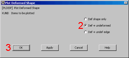
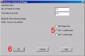
This step represents the beginning of the postprocessing phase.
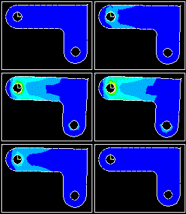
The results you see may vary slightly from what is shown due to variations in the mesh.
|
  |
|
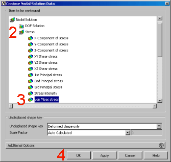
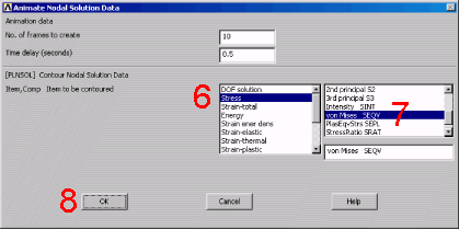
|
|
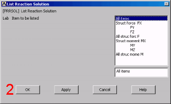 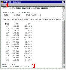 |
The value of 134.61 is comparable to the total pin load force.
The values shown are representative and may vary from the values that you obtain.
Many other options are available for reviewing results in the general postprocessor. You will see some other options in other tutorials.
You have finished the analysis. Exit the program in the next step.
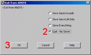
Exit the Mechanical APDL program. Upon exiting, you have the following options:
Save the geometry and loads portions of the database (default).
Save geometry, loads, and solution data (one set of results only).
Save geometry, loads, solution data, and postprocessing data (save everything).
Save nothing.
You can save nothing here, but use one of the other save options if you want to keep your data files.
|
 |


