


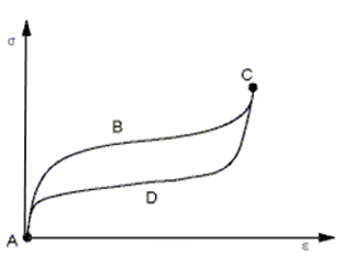
A shape memory alloy (SMA) is a metallic alloy that can undergo permanent deformation at low temperature and then recover its original shape through a phase transformation activated by increasing temperature. Upon loading and unloading cycles, an SMA can exhibit the following types of behavior:
Superelasticity (also known as pseudoelasticity) – Large deformation without residual strains.
Superelasticity and the shape memory effect occur due to the material microstructure in which two different crystallographic structures exist: austenite and martensite. Austenite is the crystallographically more-ordered phase, and martensite is the crystallographically less-ordered phase. The key characteristic of an SMA is the occurrence of a martensitic phase transformation. Shape memory effect – The material recovers its original shape through thermal cycles.
Typically, austenite is stable at high temperatures and low stress, while martensite is stable at low temperatures and high stress. The reversible martensitic phase transformation results in unique effects: the pseudoelasticity (PE) and the shape memory effect (SME). Plasticity – A permanent strain that remains in the unloaded state.
Similar to plasticity in other metals, plastic deformation in SMA materials occurs in either the austinite or martensite phase when the stress reaches the yield stress. The SMA phase transformation and plasticity are coupled through the martensite volume fraction.
The following topics about the SMA material model are available:
Also see Material Model Support for Elements for SMA. Element support varies according to the SMA material model option.
SMA material model options are available for:
Simulating superelastic behavior – Based on Auricchio et al.,[1] where the material undergoes large-deformation without showing permanent deformation under isothermal conditions.
Simulating the shape memory effect behavior of shape memory alloys – Based on the 3D thermomechanical model for stress-induced solid phase transformations of Souza et al.,[2] Auricchio et al.,[3] and Auricchio and Petrini.[4]
Combining plasticity with superelasticity and shape memory effect – A modified form of the Hartl and Lagoudas [7] model.
The following topics are available for the SMA superelasticity option:
From a macroscopic perspective, the phase-transformation mechanisms involved in superelastic behavior are:
Austenite to martensite (A->S)
Martensite to austenite (S->A)
Martensite reorientation (S->S)
Two of the phase transformations are considered here: A->S and S->A. The material is composed of two phases, the austenite (A) and the martensite (S). Two internal variables, the martensite fraction (ξS) and the austenite fraction (ξA), are introduced. One of them is a dependent variable, and they are assumed to satisfy the relation expressed as:

The independent internal variable chosen here is ξS.
The material behavior is assumed to be isotropic. The pressure dependency of the phase transformation is modeled by introducing the Drucker-Prager loading function, as follows:


where α is the material parameter, σ is the stress, and 1 is the identity tensor.
The evolution of the martensite fraction, ξS, is then defined as follows:

where:


where  are the material parameters shown in the following figure:


where  are the material parameters shown in Figure 4.58: Idealized Stress-Strain Diagram of Superelastic Behavior.
The material parameter α characterizes the material response
in tension and compression. If tensile and compressive behaviors are the same, then α =
0. For a uniaxial tension-compression test, α can be related to the initial value of
austenite to martensite phase transformation in tension and compression ( , respectively) as:

The stress-strain relation is:


where D is the elastic stiffness tensor,  is the transformation strain tensor, and
  is the material parameter shown in Figure 4.58: Idealized Stress-Strain Diagram of Superelastic Behavior.
To model the difference between the austenite and martensite elastic properties, the
elastic modulus  (used in the material constitutive model) is a function of the martensite
fraction
(used in the material constitutive model) is a function of the martensite
fraction  , the elastic modulus of pure austenite
  (the initial input elastic modulus), and the elastic modulus of pure
martensite
(the initial input elastic modulus), and the elastic modulus of pure
martensite  :
:

To model the superelastic behavior of shape memory alloys, initialize the data table via the TB,SMA command's SUPE option.
Define the elastic behavior in the austenite state (MP).
The superelastic SMA option is described by six constants that define the stress-strain behavior in loading and unloading for the uniaxial stress-state.
For each data set, define the temperature (TBTEMP), then define constants C1 through C7 (TBDATA). You can define up to 99 sets of temperature-dependent constants in the same way.
Table 4.30: Superelastic Option Constants
| Constant | Meaning | Property |
|---|---|---|
| C1 |

| Starting stress value for the forward phase transformation |
| C2 |

| Final stress value for the forward phase transformation |
| C3 |

| Starting stress value for the reverse phase transformation |
| C4 |

| Final stress value for the reverse phase transformation |
| C5 |

| Maximum residual strain |
| C6 | α | Parameter measuring the difference between material responses in tension and compression |
| C7 |

| Elastic modulus of the full martensite phase
If 0 or undefined, the martensite and austenite phases share the same elastic
modulus |

Example 4.38: Defining Elastic Properties of the Austenite Phase
MP,EX,1,60000.0
MP,NUXY,1,0.36
Define SMA material properties
TB,SMA,1,,,SUPE
TBDATA,1, 520, 600, 300, 200, 0.07, 0.0
The following topics concerning SMA and the shape memory effect are available:
The shape memory effect was based on a 3D thermomechanical model for stress-induced solid phase transformations that was presented in [2] [3][4]. Within the framework of classical irreversible thermodynamics, the model is able to reproduce all of the primary features relative to shape memory materials in a 3D stress state. The free energy potential is set to:

where:
| D = material elastic stiffness tensor |
 = total strain = total strain |
 = total transformation strain = total transformation strain |
 = deviatoric transformation strain = deviatoric transformation strain |
| τM(T) = a positive and monotonically increasing function of the temperature as 〈β(T - T0)〉+ in which 〈∙〉+ is the positive part of the argument (also known as Maxwell stress). |
| β = material parameter |
| T = temperature |
| T0 = phase-balance temperature |
| h = material parameter related to the hardening of the material during the phase transformation |
 = indicator function introduced to satisfy the constraint on the
transformation norm [1] in which = indicator function introduced to satisfy the constraint on the
transformation norm [1] in which |

from which we have


where X tr is defined as the transformation stress.
Stresses, strains, and the transformation strains are then related as follows:

Splitting the stress into deviatoric and volumetric components, we have


where S is the deviatoric stress and p is the volumetric stress (also called hydrostatic pressure)
The transformation stress is given as follows:

where γ is defined by

where  is a maximum value of
  .
.
Numerous experimental tests show an asymmetric behavior of SMA in tension and compression, and suggest describing SMA as an isotropic material with a Prager-Lode-type limit surface. Accordingly, the following yield function is assumed:

where X tr is the transformation stress, J2 and J3 are the second and third invariants of transformation stress, m is a material parameter related to Lode dependency, and R is the elastic domain radius.
J2 and J3 are defined as follows:


The evolution of transformation strain is defined as:

where ξ is an internal variable and is called as transformation strain multiplier. ξ and F(X tr) must satisfy the classical Kuhn-Tucker conditions, as follows:

which also reduces the problem to a constrained optimization problem.
The elastic properties of austenite and martensite phase differ. During the transformation
phase, the elastic stiffness tensor of material varies with the deformation. The elastic
stiffness tensor  is therefore assumed to be a function of the transformation strain
 , defined as:

where D A is the elastic stiffness tensor of austenite phase, and D S is the elastic stiffness tensor of martensite phase. The Poisson’s ratio of the austenite phase is assumed to be the same as the martensite phase. When the material is in its austenite phase, D = D A, and when the material undergoes full transformation (martensite phase), D = D S.
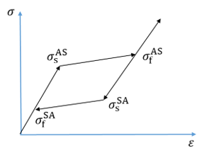
The following figure illustrates a number of the mechanical model features:
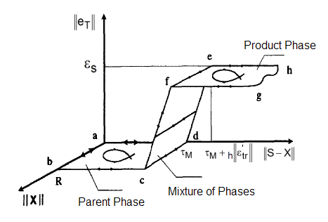
The austenite phase is associated with the horizontal region abcd. Mixtures of phases are
related to the surface cdef. The martensite phase is represented by the horizontal region efgh.
Point c corresponds to the nucleation of the martensite phase. Phase transformations take place
only along line cf, where  . Saturated phase transformations are represented by paths on line fg. The
horizontal region efgh contains elastic processes except, of course, those on line fg.
. Saturated phase transformations are represented by paths on line fg. The
horizontal region efgh contains elastic processes except, of course, those on line fg.
A backward Euler integration scheme is used to solve the stress update and the consistent tangent stiffness matrix required by the finite element solution for obtaining a robust nonlinear solution. Because the material tangent stiffness matrix is generally unsymmetric, use the unsymmetric Newton-Raphson option (NROPT,UNSYM) to avoid convergence problems.
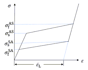
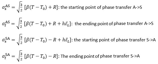
Assuming that A and S share the same elastic modulus (DS = DA) in a uniaxial loading under the constant temperature T, these are the four critical stress points (shown in Figure 4.60: Stress Points at the Start/End of the Phase Transfers) at the start and end of the phase transformations:
To model the shape memory effect behavior of shape memory alloys, initialize the data table via the TB,SMA command’s MEFF option.
Define the elastic behavior in the austenite state (MP).
The shape memory effect option is described by seven constants that define the stress-strain behavior of material in loading and unloading cycles for the uniaxial stress-state and thermal loading.
For each data set, define the temperature (TBTEMP), then define constants C1 through C7 (TBDATA). You can define up to 99 sets of temperature-dependent constants in this manner.
Table 4.31: Shape Memory Effect Option Constants
| Constant | Meaning | Property |
|---|---|---|
|
C1 |
h |
Hardening parameter |
|
C2 |
To |
Phase-balance temperature |
|
C3 |
R |
Elastic limit |
|
C4 |
β |
Temperature scaling parameter |
|
C5 |
|
Maximum value of |
|
C6 |
Em |
Martensite modulus |
|
C7 |
m |
Lode dependency parameter |


Example 4.39: Defining Shape Memory Effect Properties of the Austenite Phase
MP,EX,1,60000.0
MP,NUXY,1,0.36
Define SMA material properties
TB,SMA,1,,,MEFF
TBDATA,1,1000, 223, 50, 2.1, 0.04, 45000
TBDATA,7,0.05
This SMA model includes superelasticity, the shape memory effect, and plastic yielding.
Following a small-strain formulation, the total strain  is additively decomposed through:

in terms of the elastic strain  , thermal strain
  , transformation strain
  , and plastic strain
  . The transformation strain is decomposed into a magnitude and direction
through:
. The transformation strain is decomposed into a magnitude and direction
through:

where:
 = material parameter characterizing the maximum transformation
strain = material parameter characterizing the maximum transformation
strain |
 = volume fraction of martensite constrained to the range of [0,1],
representing the formation and depletion of all martensite variants = volume fraction of martensite constrained to the range of [0,1],
representing the formation and depletion of all martensite variants |
 = direction of the transformation strain constrained to have a unit magnitude
(that is, = direction of the transformation strain constrained to have a unit magnitude
(that is,  ) ) |
The foundation of the model is the Helmholtz free-energy function, assumed to take the form:

The elastic part contains:
 = phase-dependent bulk modulus = phase-dependent bulk modulus |
 = total volumetric strain = total volumetric strain |
 = phase-dependent shear modulus = phase-dependent shear modulus |
 = total deviatoric strain = total deviatoric strain |
 = coefficient of thermal expansion = coefficient of thermal expansion |
 = temperature (absolute). (The program
adds the offset temperature [TOFFST] to all temperatures and corresponding
coefficients.) = temperature (absolute). (The program
adds the offset temperature [TOFFST] to all temperatures and corresponding
coefficients.) |
 = reference temperature for thermal
expansion = reference temperature for thermal
expansion |
The thermal energy contains:
 = phase-balance temperature (at which
the specific free energies of the two phases are the same at stress-free conditions)
(absolute) = phase-balance temperature (at which
the specific free energies of the two phases are the same at stress-free conditions)
(absolute) |
 is an internal variable providing a lower bound for is an internal variable providing a lower bound for  |
 = entropy difference during transformation = entropy difference during transformation |
Note:
 during forward transformation, and
  during reverse transformation.
The interaction part contains:
 = hardening energy = hardening energy |
 = transformation hardening parameter = transformation hardening parameter |
The constraint energy is defined using:
 = Lagrange multipliers (which enforce the constraints = Lagrange multipliers (which enforce the constraints  and and  , respectively) , respectively) |
The plastic energy contains:
 = linear kinematic hardening modulus (phase-independent) = linear kinematic hardening modulus (phase-independent) |
Both the bulk and shear moduli are dependent on the phase through a Reuss homogenization approach using:
 |
with  representing the value in austenite and
  the value in martensite.
The definitions of  can be obtained from the material parameters
  through the following:
 |
 |
Using the Helmholtz free-energy function, the stress is:

Considering a constant  , the dissipation function for transformation is assumed to take on the form
of:
, the dissipation function for transformation is assumed to take on the form
of:
 |
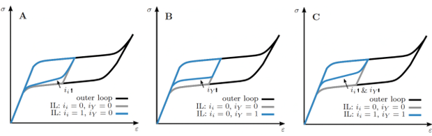
where  represents the radius of the elastic domain of transformation. The parameter
 controls the width of the hysteresis of the outer loop, while
  changes the hysteresis for the internal loops. The factor
  modifies the radius of the elastic domain based on the amount of phase
available for transformation. The available phase is defined based on the memory points as
modifies the radius of the elastic domain based on the amount of phase
available for transformation. The available phase is defined based on the memory points as
 for reverse transformation and
  for forward transformation.
The transformation hardening energy  is defined through its derivative with respect to
  :
:
 |
 additionally accounts for the smooth development of internal (or minor) loops
in the case of incomplete transformations using:
additionally accounts for the smooth development of internal (or minor) loops
in the case of incomplete transformations using:
 |
with the hardening function for the outer (or major) loop  , the hardening function for the internal loop
  and a factor
  for adjusting the internal loop feature. The outer loop hardening is described
using a polynomial function:
for adjusting the internal loop feature. The outer loop hardening is described
using a polynomial function:
 |
Here, the factors  and
and  describe the offset of the transformation stress from that of a linear
response near the beginning and end of transformation, and
describe the offset of the transformation stress from that of a linear
response near the beginning and end of transformation, and  is a linear hardening factor.
  and
and  affect the curvature of the hardening process near the beginning and end of
transformation.
affect the curvature of the hardening process near the beginning and end of
transformation.
The internal loop hardening function is represented based on a scaling
of the outer loop hardening based on the memory points  and
and  . During forward transformation the internal loop factor
  and the internal loop transformation hardening
  are obtained as
 |
Similarly, during reverse transformation the relevant variables are defined by
 |
The internal loop factor depends on a material parameter  for turning the internal loop behavior on or off.


The thermodynamic force associated with plasticity is defined as:
 |
The limit function for the plasticity is considered to be phase and stress-state dependent through the expressions:
 |
 |
 |
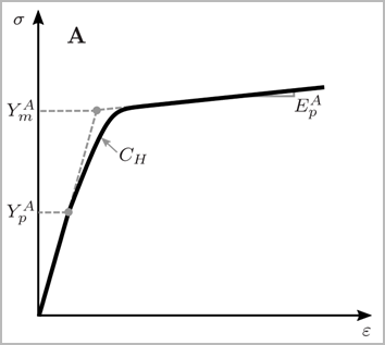
Here,  is a nonlinear isotropic hardening function decomposed into an austenite
 part and a martensite
  part.
part.  is a function to introduce tension-compression asymmetry through a dependence
on the transformation strain direction
is a function to introduce tension-compression asymmetry through a dependence
on the transformation strain direction  . The material parameter
  defines the factor of increase in the isotropic hardening and yield point for
the plasticity in compression compared to tension. For tension-compression symmetric behavior,
defines the factor of increase in the isotropic hardening and yield point for
the plasticity in compression compared to tension. For tension-compression symmetric behavior,
 is set to 1. The nonlinear isotropic hardening functions are dependent on the
phase using:
is set to 1. The nonlinear isotropic hardening functions are dependent on the
phase using:
 |
 |
where  is the initial yield point of austenite and
  is the initial yield point of martensite. The isotropic hardening becomes
saturated to the yield point
is the initial yield point of martensite. The isotropic hardening becomes
saturated to the yield point  for austenite and
  for martensite. The isotropic linear hardening following the exponential
hardening is defined through
for martensite. The isotropic linear hardening following the exponential
hardening is defined through  and
and  for austenite and martensite, respectively. The parameter
  determines how rapidly the saturation from
  to
to  and
and  to
to  takes place.
  is the accumulated equivalent plastic strain.
The function  is the basis for the tension-compression asymmetry and is defined as:
 |
where the internal parameters  ,
,  , and
, and  define the tension-compression asymmetric surface and
  . The internal parameters are chosen such that the function
  can achieve maximum asymmetry while remaining convex. The maximum
transformation strain can be made tension-compression asymmetric using:
can achieve maximum asymmetry while remaining convex. The maximum
transformation strain can be made tension-compression asymmetric using:
 |
in terms of the maximum transformation strain in tension  and the maximum transformation strain in compression
  . Similarly, the Young’s modulus of martensite can be made
tension-compression asymmetric using:
. Similarly, the Young’s modulus of martensite can be made
tension-compression asymmetric using:
 |
in terms of the Young's modulus of martensite in tension  and compression
  .
.
Figure 4.63: Stress-strain curve displaying tension-compression behavior of the maximum transformation strain and the Young’s modulus of martensite
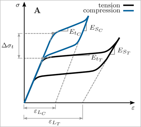
If values for the corresponding parameters are not defined, then default values are used so that the tension and compression behavior of the material are the same.
Note that the tension-compression asymmetry feature is optional. If
this feature is not enabled, the model is symmetric in tension and compression.
Tension-compression asymmetry is activated for the maximum transformation strain and the Young's
modulus of martensite by defining  and
and  , respectively. In that case, the input parameters
  and
and  are set to
  and to
  , respectively. The internal loop behavior is also optional.
The material tangent-stiffness matrix is unsymmetric for this material model, so it can be beneficial to use the unsymmetric Newton-Raphson solution option (NROPT).
The austenite phase elastic behavior is defined with the material
elastic constants (TB or MP). Initialize the data table
(TB,ELAS) and define the Young's modulus of austenite ( ) and the Poisson's ratio (
 ). Alternatively, use MP,EX to define the Young's modulus
of austenite and MP,PRXY/NUXY to define the Poisson's ratio. The austenite
phase elastic behavior is assumed to be isotropic.
). Alternatively, use MP,EX to define the Young's modulus
of austenite and MP,PRXY/NUXY to define the Poisson's ratio. The austenite
phase elastic behavior is assumed to be isotropic.
To define the constants, initialize the data table
(TB,SMA) with options (TBOPT) METE, METL, METH,
MEPD, and METC. The function of each option follows:
| METE (required) -- Defines the martensite phase elastic response and thermal expansion. |
| METL (required) -- Specifies the limits of transformation in strain-stress-temperature space and thus defines the phase diagram of a given SMA material. |
METH (required) -- Considers the smooth behavior of
transformation by applying a hardening function for the evolution of the martensite volume
fraction  . . |
| MEPD (required) -- Defines the plastic phase-dependent yielding response. The plasticity exhibits linear kinematic and nonlinear isotropic hardening. |
| METC (optional) -- Defines the tension-compression asymmetry response and hysteresis response. If not defined, the program determines default parameter values. |
For each data set, define temperature- and field-dependence (TBFIELD), if any, then define the material parameters (TBDATA) as shown in the following tables:
Table 4.32:
TBDATA Constants for
TB,SMA,,,,TBOPT = METE
| Constant | Meaning | Property | Range |
|---|---|---|---|
| C1 |

| Young’s modulus of martensite |

|
| C2 |

| Thermal expansion coefficient |

|
Table 4.33: TBDATA Constants for
TB,SMA,,,,TBOPT = METL
| Constant | Meaning | Property | Range |
|---|---|---|---|
| C1 |

| Maximum transformation strain |

|
| C2 | 
| Phase-transformation limit |

|
| C3 |  | Phase-balance temperature |  |
| C4 | 
| Entropy difference for forward transformation |

|
| C5 |
 | Entropy difference for reverse transformation |

|
Table 4.34:
TBDATA Constants for
TB,SMA,,,,TBOPT = METH
| Constant | Meaning | Property | Range |
|---|---|---|---|
| C1 |

| Transformation hardening modulus | |
| C2 |

| Transformation hardening factor |

|
| C3 |

| Transformation hardening factor |

|
| C4 |

| Transformation hardening factor |

|
| C5 |

| Transformation hardening exponent |

|
| C6 |

| Transformation hardening exponent |

|
Table 4.35:
TBDATA Constants for
TB,SMA,,,,TBOPT = MEPD
| Constant | Meaning | Property | Range |
|---|---|---|---|
| C1 |
 | Isotropic hardening modulus of austenite |

|
| C2 |
 | Isotropic hardening modulus of martensite |

|
| C3 |
 | Isotropic plastic yield point of austenite |

|
| C4 |
 | Isotropic plastic yield point of martensite | 
|
| C5 |  | Isotropic plastic yield saturation point of austensite |

|
| C6 |

| Isotropic plastic yield saturation point of martensite |

|
| C7 |
 | Isotropic plastic yield saturation rate parameter |

|
| C8 |  | Kinematic hardening modulus |  |
Table 4.36:
TBDATA Constants for
TB,SMA,,,,TBOPT = METC
| Constant | Meaning | Property | Range | Default |
|---|---|---|---|---|
| C1 |  | Young’s modulus of martensite in compression |  |  |
| C2 |  | Maximum transformation strain in compression |  |  |
| C3 |  | Compression plasticity factor (the ratio of the compression-yield point to the tension-yield point) |  | 1 |
| C4 |  | Hardening internal loop factor |  | 0 |
| C5 |  | Hysteresis internal loop factor |  | 0 |
Example 4.40: Defining the Shape Memory Effect Properties of the Austenite Phase
!================================================!
! Material parameters for SMA plasticity model
!================================================!
! Thermo-elasticity
C1 = 37700      !EA
C2 = 31800      !ES
C3 = 0.33       !nu
C4 = 0.0        !alpha
! Transformation limits
C5 = 0.041      !eL
C6 = 259        !YS
C7 = 261        !theta0
C8 = 6.4        !deletaf
C9 = 9.4        !deletar
! Transformation hardening
C10= -9000      !mut
C11= -70        !a1
C12= 300        !a2
C13= 9500       !a3
C14= 30         !n1
C15= 30         !n2
! Plasticity
C16= 1000       !hpA
C17= 1000       !hpS
C18= 1000       !YpA
C19= 1000       !YpS
C20= 1200       !YmA
C21= 1200       !YmS
C22= 200        !CH
C23= 14000      !mup

TB,ELAS,1
TBDATA,1,C1,C3
TB,SMA,mat1,,,METE
TBDATA,1,C2,C4
TB,SMA,mat1,,,METL
TBDATA,1,C5,C6,C7,C8,C9
TB,SMA,mat1,,,METH
TBDATA,1,C10,C11,C12,C13,C14,C15
TB,SMA,mat1,,,MEPD
tbdata,1,C16,C17,C18,C19,C20,C21
tbdata,7,C22,C23
The default temperature unit is Kelvin. If using another temperature unit, the corresponding coefficients for the constants need to be converted. This table shows how to convert a given coefficient value from one temperature-unit system to another:


For postprocessing, solution output is as follows:
Stresses are output as S.
Elastic strains are output as EPEL.
For the superelasticity (SUPE) and shape memory effect (MEFF) SMA model options:
Transformation strains are output as EPPL.
The value of
 is available as part of nonlinear solution record NL and can be processed
as component EPEQ of NL.
is available as part of nonlinear solution record NL and can be processed
as component EPEQ of NL.
For the shape memory effect with plastic deformation (METE+METL+METH+MEPD) SMA model option:
EPPL represents the plastic strain.
Transformation strain is output as EPCR.
EPEQ of NL represents the accumulative equivalent plastic strain.
Elastic strain energy density is available as part of the strain energy density record SEND (ELASTIC).
Auricchio, F. (2001). A robust integration-algorithm for a finite-strain shape-memory-alloy. International Journal of Plasticity. 17, 971-990.
Souza, A. C., Mamiya, E. N., & Zouain, N. (1998). Three-dimensional model for solids undergoing stress-induced phase transformations. European Journal of Mechanics-A/Solids. 17, 789-806.
Auricchio, F., Taylor, R. L., & Lubliner, J. (1997). Shape-memory alloys: Macromodeling and numerical simulations of the superelastic behavior. Computational Methods in Applied Mechanical Engineering. 146(1), 281-312.
Auricchio, F. & Petrini, L. (2005). Improvements and algorithmical considerations on a recent three-dimensional model describing stress-induced solid phase transformations. International Journal for Numerical Methods in Engineering. 55, 1255-1284.
Auricchio, F., Fugazza, D., DesRoches, R. (2006). Numerical and experimental evaluation of the damping properties of shape-memory alloys. Journal of Engineering Materials and Technology. 128(3), 312-319.
Hartl, D. J., & Lagoudas, D. C. (2009). Constitutive modeling and structural analysis considering simultaneous phase transformation and plastic yield in shape memory alloys. Smart Materials and Structures. 18(10), 1-17.
Woodworth, L.A., Wang, X., Lin, G., & Kaliske, M. (2022). A multi-featured shape memory alloy constitutive model incorporating tension-compression asymmetric interpolation. Mechanics of Materials. 172.
For an example analysis, see Shape Memory Alloy (SMA) with Thermal Effect in the Technology Showcase: Example Problems.