This example is based on a generic composite wind blade with variable cross section, realistic subcomponents, materials, and thickness distribution. It is used as the base to compute the equivalent beam properties. A modal analysis is run on the equivalent beam model and its frequencies are compared against the 3D Shell model frequencies (SHELL181 elements).
 The fully
configured Workbench project is contained in a compressed file and can be downloaded
here. This configured project requires Release 2025 R1 or more recent
versions.
The fully
configured Workbench project is contained in a compressed file and can be downloaded
here. This configured project requires Release 2025 R1 or more recent
versions.
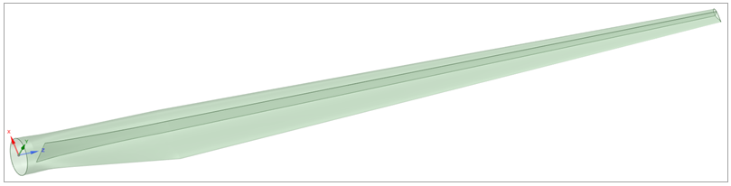
The blade has a circular root section that transitions to aerodynamics airfoil. Its structure mimics a typical wind blade with longitudinal UD spar caps, a shear web, trailing edge UD reinforcement, +/- 45 external skins, and core material in the panels.
The material properties are listed in the table below.
Table 4.3: Material Properties
| Foam | Glass UD | |
| Ex [Mpa] | 70 | 45000 |
| Ey [Mpa] | 70 | 10000 |
| Ez [Mpa] | 70 | 10000 |
| Gxy [Mpa] | 26.92 | 5000 |
| Gxz [Mpa] | 26.92 | 5000 |
| Gyz [Mpa] | 26.92 | 5000 |
| νxy | 0.3 | 0.3 |
| νxz | 0.3 | 0.3 |
| νyz | 0.3 | 0.4 |
| Density [t/mm3] | 6E-11 | 2.0E-09 |
The blade is 50.6 m long and, due to the variable cross section and design, the beam model has 101 elements. This means that the sectional properties have to be calculated at 101 locations. Ideally, the section cuts are in the middle of each section cut.
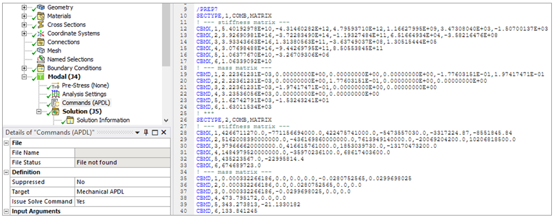
There are two Python scripts in the ACP model. The first is to generate the section cuts at the right locations (middle of each beam element). And the second script is to write the results as sectional properties to an APDL input file. The script is based on the example [Export Section Cut]. The generated output must be manually copied into the APDL Command snippet or refresh the Command snippet to load it directly from the generated APDL input file.
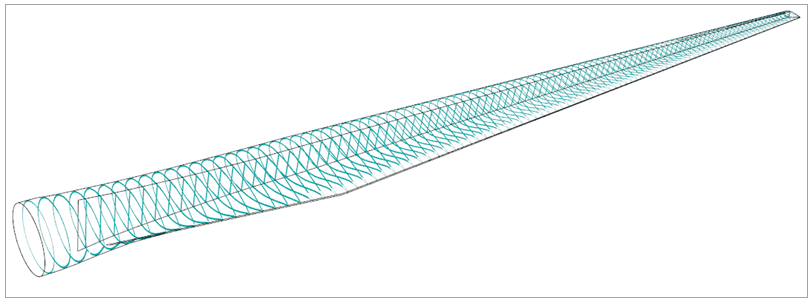
Figure 4.70: Two Meshes of Different Cross Sections and the Corresponding Shear, Elastic, and Center of Gravity
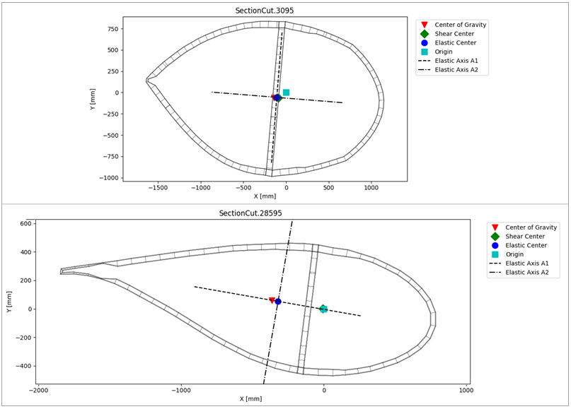
For this example, the reference point considered for the cross section properties is the Origin. The Mesh (nodes and elements) for the beam model is created conveniently in Mechanical APDL to place the nodes at the desired location along the span of the blade. Then, this model is imported into the Workbench application via an external model (.cdb) and can be opened in the Mechanical application, where using an APDL snippet, each element property is reassigned according to the calculated values for each cross section (these values were saved through the ACP Python script into a .cdb file)
The blade is fixed on one hand and the first five frequencies are calculated. The table below compares the results of the 3D shell model and equivalent beam model.
Table 4.4: Comparison of the 3D Shell Model and Equivalent Beam Model Results
| Shell | Equivalent Beam | Mode Shape | Diff. % |
| 0.66264 | 0.67738 | First flap | 2.2% |
| 0.69092 | 0.70684 | First edge | 2.3% |
| 2.3553 | 2.3932 | Second flap | 1.6% |
| 3.2611 | 3.32467 | Second edge | 1.9% |
| 5.3698 | 5.472 | Third flap | 1.9% |
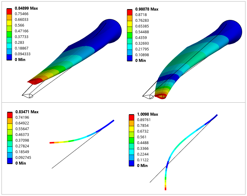
The following figure shows a comparison of the mode shapes for the first and fourth frequencies.
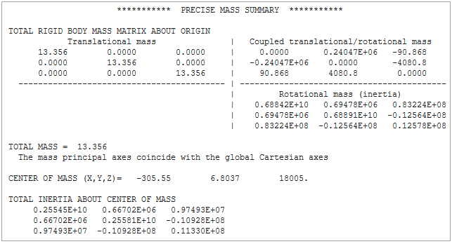
You may compare the data of the inertia properties for the 3D solid model and equivalent beam model using the reports below.
Shell Model
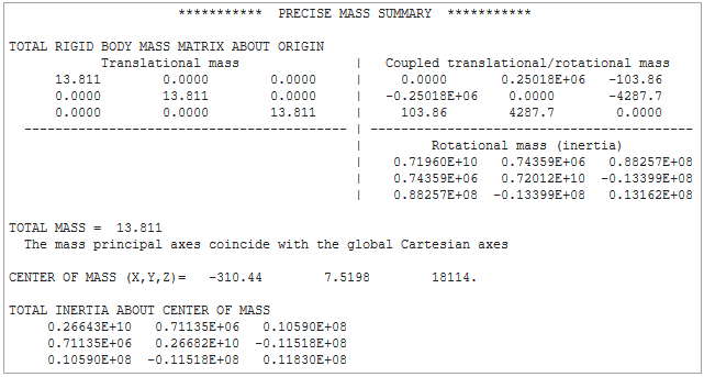
Equivalent Beam Model