There are several features that can be used for viewing the results of a simulation. They all can give a different insight into the behavior of the composite structure. The different postprocessing visualizations mentioned below are also described in the last part of Tutorial 1.
Composites are significantly more complex than isotropic materials because of their orthotropic material behavior and multiple possible failure modes (different types of fiber, matrix failure, etc.). Therefore, composites are evaluated based on standard results (such as deformation, stress, and strain) and on failure criteria to identify the first ply failure of the structure.
This section describes the use of the standard result objects in the Mechanical software for composite, ply-wise scoping, and failure criteria evaluation.
Deformation
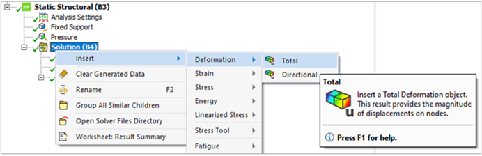
In the Mechanical application, you can visualize the deformation of a structure with the following result objects: Total Deformation or Directional Deformation. The Display Time field in the Details panel enables you to plot the result at a specific time. The plot can be scaled by using the Deformation Scale in the Result tab's Display group.

Failure Criteria
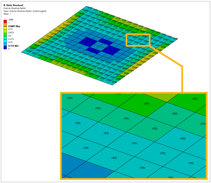
The failure plot displays the critical safety factors (reserve factors, inverse reserve factors, and margin of safety) to first ply failure for a given failure criteria definition.
The safety factors are evaluated for every element of each layer and the critical value through the thickness of the lay-up is then projected on to the reference shell mesh. A failure plot for an envelope solution works in the same way and is a display of the most critical failure of all included solution sets. Alternatively, the safety factors can be displayed ply-wise for each analysis ply.
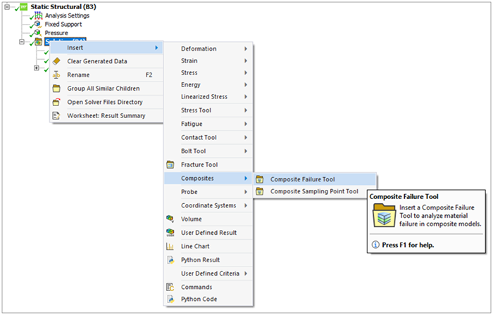
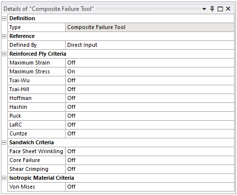
Before creating a failure plot, you must insert a Composite Failure Tool under the Solution and complete the failure criteria definition.
You can insert a Composite Failure Tool by right clicking the Solution group object, navigating to the Composites cell, and selecting the Composite Failure Tool.
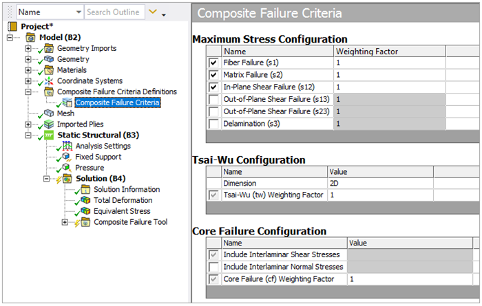
When you click the Composite Failure Tool group object, you can enable/disable the failure criteria in its Details panel. The failure criteria definition (such as the IRF) must be performed before creating the failure plot. When creating the failure criteria group, the IRF is inserted by default.
Additionally, you can display the critical failure modes and critical plies as element labels. To configure the display setup, select the result object (for example, IRF) under the Composite Failure Tool and modify the respective fields in the Details panel.
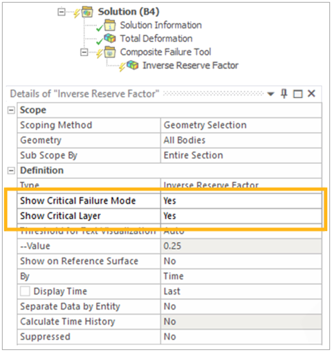
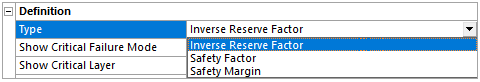
In the Details panel, you may also change the Type of failure (Inverse Reserve Factor, Safety Factor, Safety Margin).
You can view and zoom in on the results.
Ply-Wise Results
The structural behavior throughout the lay-up at each layer is of great interest in composite design. Ply-wise information helps to identify and optimize layers that are critical and ones that are not.
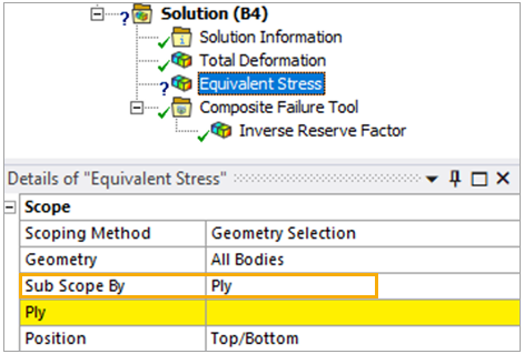
All the solution plots except the deformation plot have the option of displaying results ply-by-ply. If a result object supports ply-scoping, then the Sub Scope By field will be exposed in the Details panel. Its options are Layer and Ply. To postprocess across the entire envelope of the selected geometries, select Layer. To evaluate only a selected ply, select Ply.
Evaluate the ply-wise results through the following steps:
In the respective solution plot Details panel, select Ply as the definition of the Sub Scope By field.
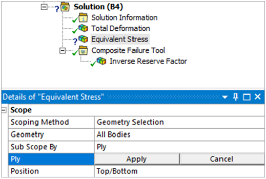
Select the respective Ply field.
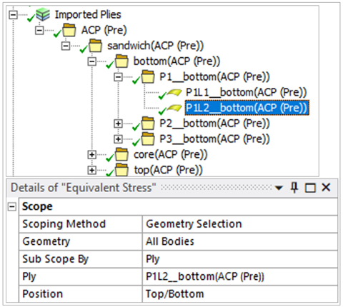
Navigate to the Imported Plies group and select the desired ply.
Return to the result object's Ply field and click Apply.
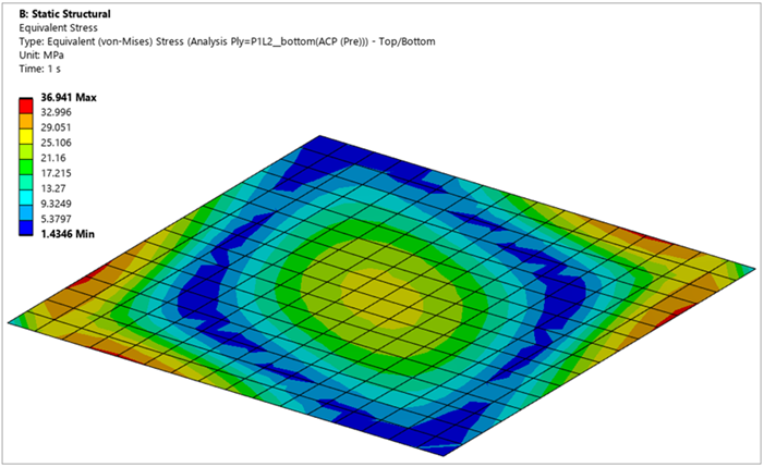
The result object can now be evaluated on the selected ply.
Sampling Point Results
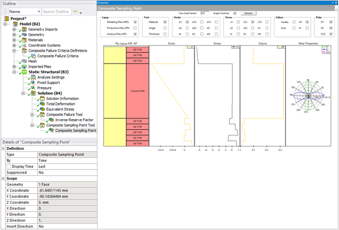
Sampling Points are an alternative way of analyzing a lay-up on a ply level. A point of interest on the composite part is selected and its local lay-up is sampled. This feature can display failure criteria, stresses, and strains through the thickness of the laminate. In this way, the Sampling Point gives a detailed insight into the laminate behavior ply-by-ply.
Insert and evaluate a Sampling Point result through the following steps:
Insert a Composite Failure Tool group object and define the Failure Criteria using the steps explained in the Failure Criteria section.
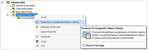
Select the Composite Failure Tool group, then right-click and select the Promote to Composite Failure Criteria cell. That places a Composite Failure Criteria Definitions group under the Model in the Tree View, which contains the user-defined Composite Failure Criteria object.
In the Details panel of the Composite Failure Tool, the Defined By field now contains Composite Failure Criteria Definitions instead of Direct Input. This enables the Failure Tool to refer to the Criteria Definitions group for the Failure Criteria definition. By default, the promoted Composite Failure Criteria object is selected.
The Composite Failure Criteria objects under the Composite Failure Criteria Definitions group can be modified, and the Failure result objects under the Solution which refer to them will be updated accordingly.
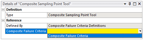
Right-click the Solution group object, navigate to the Composites field, and select the Composite Sampling Point Tool.
In the Details panel of the Composite Sampling Point Tool, select the promoted Composite Failure Criteria.
You can now choose a point and evaluate:
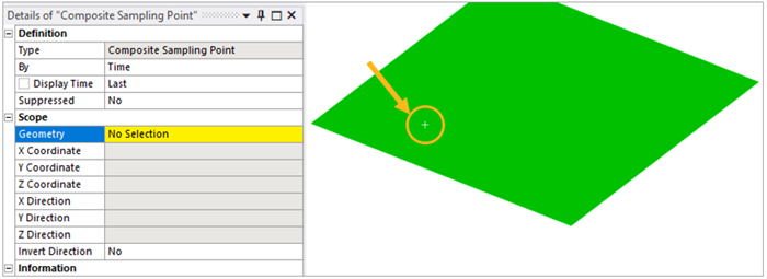
Select the Composite Sampling Point result object that has been automatically created under the respective group.
Click the Geometry field which is currently undefined.
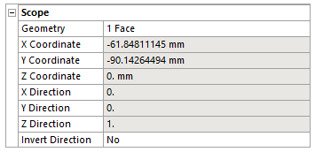
Click any area of the Geometry and then Apply. The white cross on the Geometry represents the selected point.
The details of the selected point are reported under the Scope group of the object. You can redefine the point by navigating to the Geometry, selecting another target, and re-applying the selection.
After evaluating the result, the Worksheet view is activated, where you can select which type of layup to postprocess, the results (strain, stress, failure, and polar of the material), and annotation. You can also scale the core to modify the layup plot visualization.