In this section, you will explore more postprocessing options with the Mechanical application.
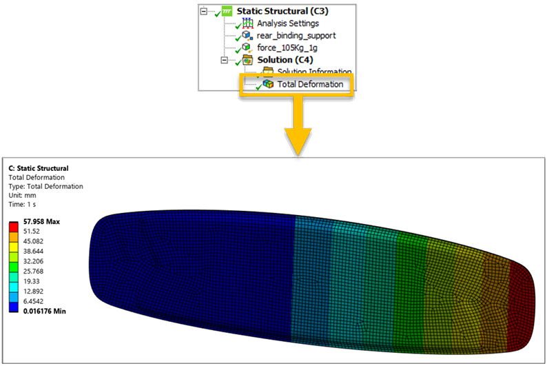
Follow these steps to create a deformation plot using the Total Deformation object:
In the tree Outline, right-click Solution and select Insert. Select Deformation, then click Total.

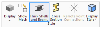
Switch to the Display tab, then select Thick Shells and Beams in the Style group.
Right-click Total Deformation object and select Retrieve This Result to visualize the plot.
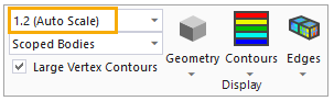
Note: The default deformation scale is 1.2 (Auto Scale). You can view and change this by navigating to the Display group of the Result tab.
In the Mechanical application, you can create stress plots for the composite model and individual Analysis Plies. You can also view the stress value at any point or locate the minimum/maximum value on an object. Finally, it is possible to view different plot results when you insert another stress type or change the component.
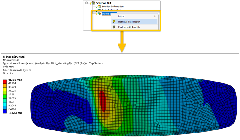
In the following example, the Normal Stress across the Fiber’s X-direction for the bottom Analysis Ply will be evaluated:
In the Tree View, right-click the Solution group and select Insert > Stress > Normal Stress.

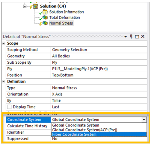
In the Details panel of the Normal Stress object, select the undefined Ply field. Then, expand the Imported Plies group, select the bottom ply of the structure (P1L3_ModelingPly.1(ACP(Pre)), and click Apply to define that selection field.

In the Details panel of the Normal Stress object, expand the list of the Coordinate System field and select the Fiber Coordinate System for postprocessing.
To postprocess the result, right-click the Normal Stress object and select Retrieve This Result.
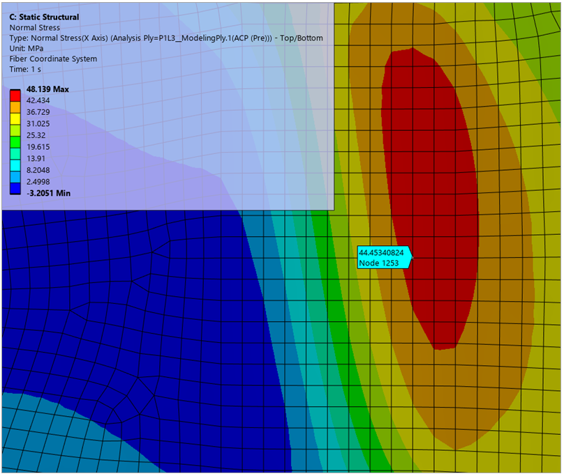
You can use the Probe tool from the Result tab to select a specific node and evaluate the result.
Tip: You can change the stress type and component by modifying Type and Orientation in the Details panel of the Stress object.
Similar to stress plots, failure plots enable you to examine the failure result of the whole structure, separate layers, or individual elements. You can also examine the failure modes, check on which plies the critical failures occur, and modify the plot legend.
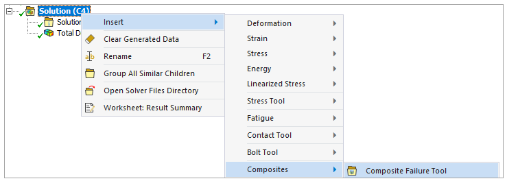
Follow these steps to create a failure plot using the Composite Failure Tool object:
In the tree Outline, right-click Solution and insert a Composite Failure Tool under Composites.
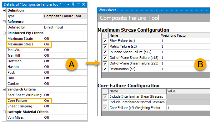
In the Details pane, switch Maximum Stress and Core Failure to On (A). In the Worksheet pane, configure the Maximum Stress and Core Failure properties as shown in the image below (B).
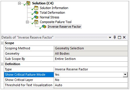
Expand Composite Failure Tool under Solution to check the Inverse Reserve Factor.
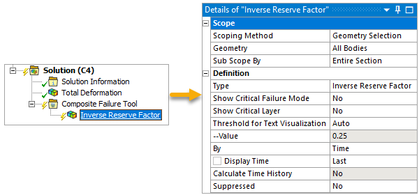
Right-click Inverse Reserve Factor and select Retrieve This Result to view the Composite Failure plot.
Note: You can use probes to identify result quantities at any point or locate the minimum/maximum value on an object. To do the former, select the result plot of interest, then go to the Result tab, click the Probe icon, and hover over the plot to obtain the result values. You can also click the object to create a probe annotation for the location of interest. To do the latter, go to the Result tab, click the Maximum and/or Minimum icon in the toolbar, and then select the result plot of interest.
Tip: Similar to the workflow for the Normal Stress result, you can enable as the method of the Sub Scope By field to view the failure results layer by layer.
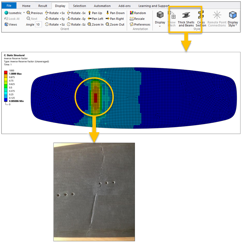
Next, you can visualize the results in a 2D projection of the structure and evaluate the failure modes and critical layers:
Navigate to the Display tab and disable the Thick Shell and Beams option.
In the Details panel of the Inverse Reserve Factor result object, activate the Show Critical Failure Mode field by setting it to Yes.
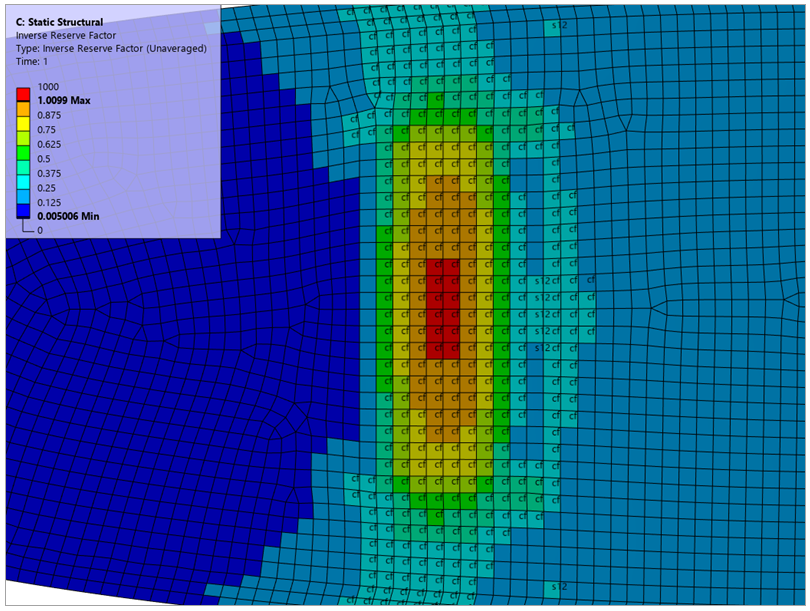
Evaluate the result to see the failure modes in the model.
Note: Failure Mode Notations
Maximum Strain e1t, e1c, e2t, e2c, e12 Maximum Stress s1t, s1c, s2t, s2c, s3t, s3c, s12, s23, s13 Tsai-Wu 2D and 3D tw Tsai-Hill 2D and 3D th Hashin
hf (fiber failure)
hm (matrix failure)
hd (delamination failure)
Puck (simplified, 2D and 3D)
pf (fiber failure)
pmA (matrix tension failure)
pmB (matrix compression failure)
pmC (matrix shear failure)
pd (delamination)
LaRC (2D)
lf (fiber failure)
lmt (matrix failure tension)
lmc (matrix failure compression)
Cuntze 2D and 3D
cft (fiber tension failure)
cfc (fiber compression failure)
cmA (matrix tension failure)
cmB (matrix compression failure)
cmC (matrix wedge shape failure)
Sandwich Failure Wrinkling
wb (wrinkling bottom face)
wt (wrinkling top face)
Sandwich Failure Core cf (core failure) Hoffman ho e = strain
s = stress
1 = material 1 direction
2 = material 2 direction
3 = out-of-plane normal direction
12 = in-plane shear
13 and 23 = out-of-plane shear terms
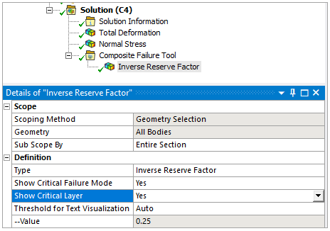
In the Details panel of the Inverse Reserve Factor, activate the Show Critical Layer field by setting it to Yes.
Zoom into the failure area of the model. The plot still shows the failure across all plies, but the annotation indicates that the core failures occur on ply 4.
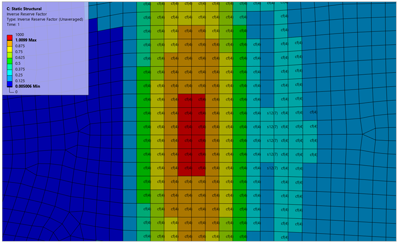
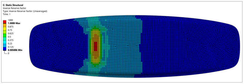
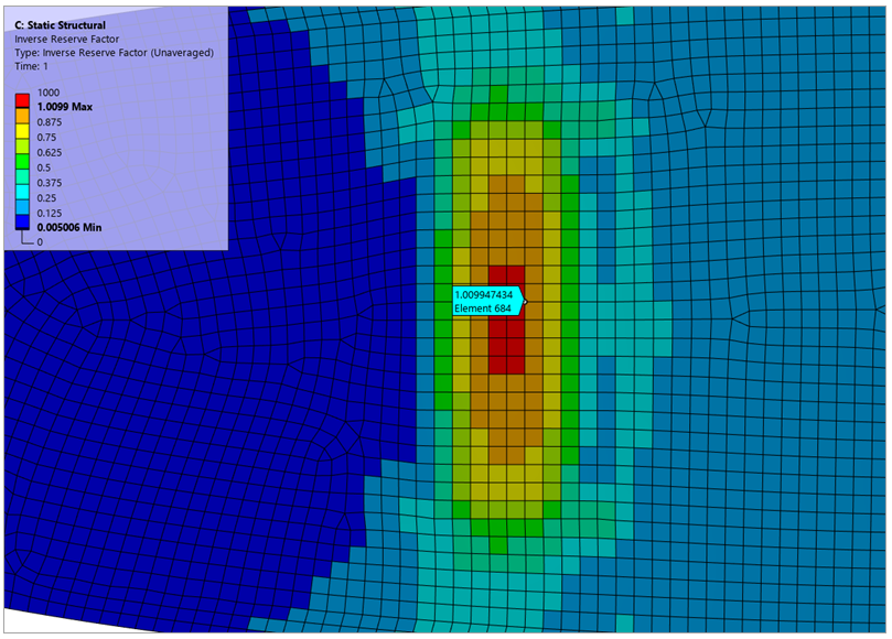
Activate the Probe feature from the Result tab, then hover over an element and select a corner node to view the exact failure value of that element. The maximum inverse reserve factor (Irf) value of this model is 1.0099 (A, below). However, the legend shows a maximum of 1000 (B).
Right-click a number on the Legend and select Adjust to Visible.
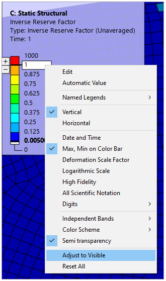
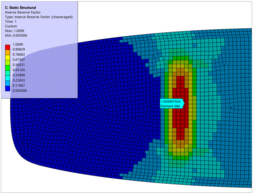
This results in more accurate maximum and minimum values on the legend.
To create a through-the-thickness plot to analyze a particular sampling point, follow these steps:
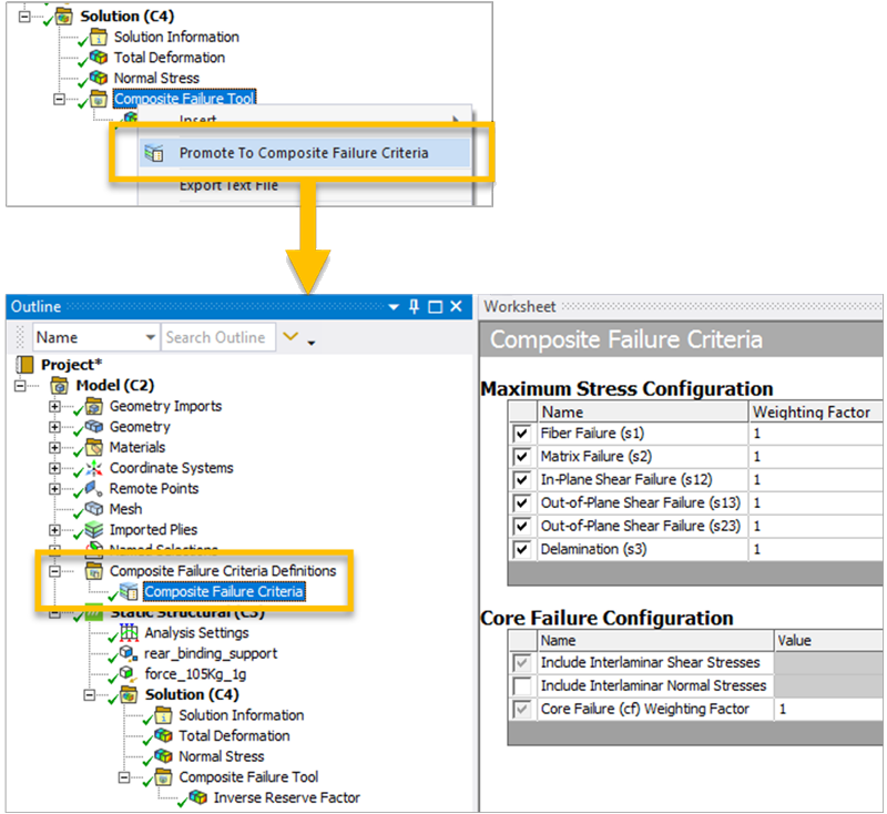
Select the Composite Failure Tool group, right-click, and select Promote to Composite Failure Criteria. This will create a group named Composite Failure Criteria Definitions under the Model in the Tree View, which contains the user-defined Composite Failure Criteria objects.
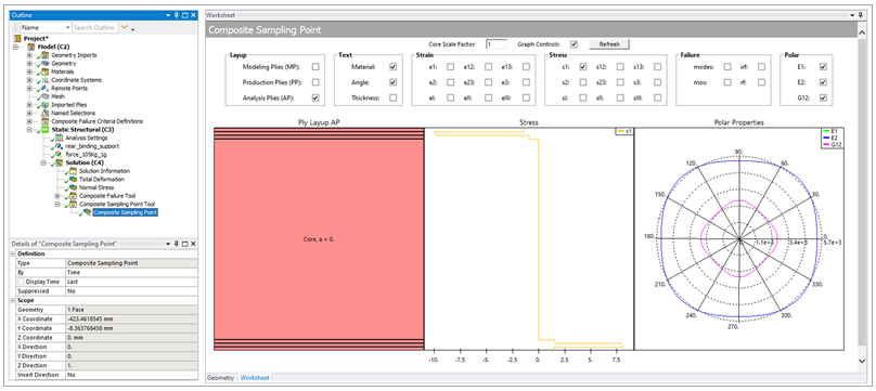
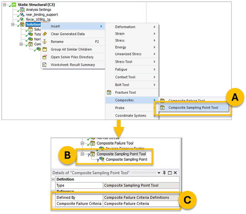
Right-click the Solution group and select Insert > Composites > Composite Sampling Point Tool (A, below).
In the Details panel of the Composite Sampling Point Tool (B), set the Composite Failure Criteria field (C) to the newly promoted Composite Failure Tool's criteria.
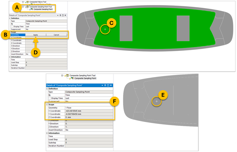
Switch to the Composite Sampling Point object (A), click the undefined Geometry field (B), select a point in the Model (C), and click Apply (D). The white cross (E) represents the location of the selected Sampling Point which can also be seen under the Scope group of the object (F).
After evaluating the result, you can view the Worksheet of the object and select which items to postprocess. To analyze the results for the selected Sampling Point, enable the items shown below.