Only acoustic boundary conditions and loads are applied, as the model uses only acoustic elements. Structural members are ignored in this example, but their effect on the model is retained through rigid outer boundaries of the back cavity and absorbing tubes. Note that rigid wall (Neumann boundary) behavior is applied as default in acoustic formulations as this is a natural boundary condition in the finite element formulation.
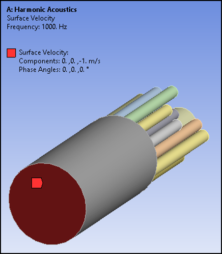
A normal surface velocity is applied on the exterior face. A transparent port and a radiation boundary are also applied on the same face:
Another port, required to calculate the absorption coefficient, is defined on the end faces of all the tubes.
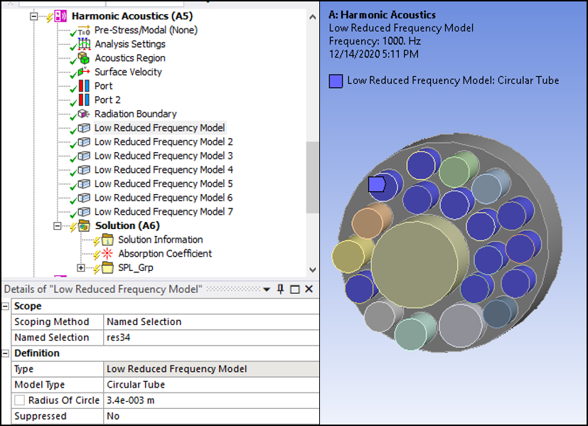
For the LRF model, geometric details of the thin channel are needed like the absorbing tube radii in this example. In the first Harmonic Acoustics system, separate LRF models are applied for each radius group with the radius specified property in the details of the LRF model object using available Named Selections as the scoping method. (Named Selections have been previously added for groups of tubes with similar radii.) The following image shows LRF model applied on bodies having radius 3.4 mm.
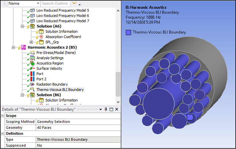
In the second Harmonic Acoustics system, a single Thermo-Viscous BLI boundary is applied on all faces (cylindrical and circular) of tubes with the settings shown in the following figure.