


In turbomachinery engineering, the hot-to-cold method is commonly used to design rotor blades. The rotor blade geometry that would represent the as-manufactured shape is referred to as the cold geometry, whereas the shape of the rotor blade in the running condition is termed the hot geometry.
The designer begins with the hot geometry of the blade and determines the final shape of the hot geometry via design optimization. Based on the desired hot geometry, the designer then uses an iterative approach to obtain the cold geometry of the blade to manufacture. The following figure illustrates a typical work flow of the iterative approach for a simple beam model.
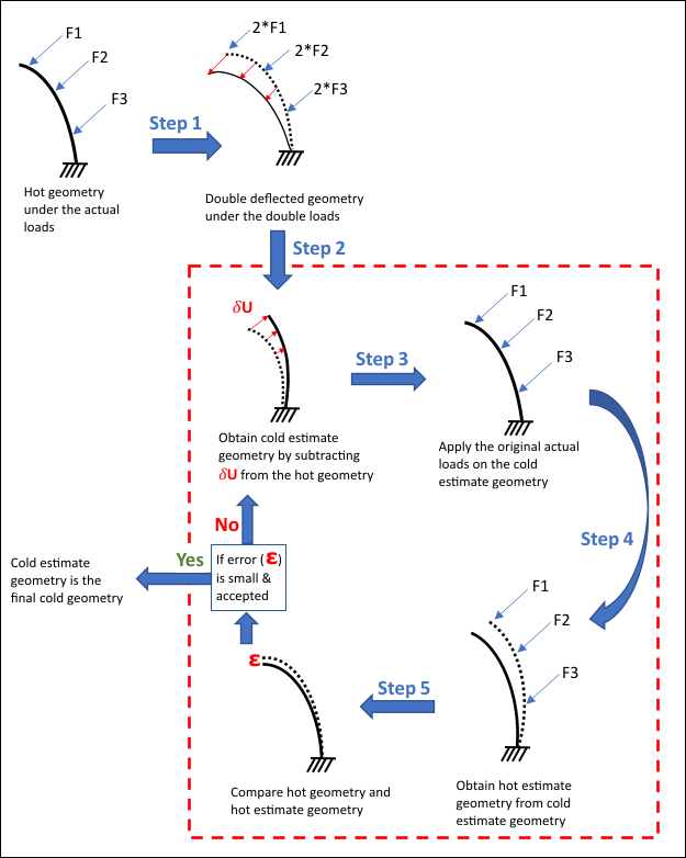
The steps of the iterative approach are as follows:
Solve the hot geometry again with the aerodynamic, centripetal, and other loads to obtain the double-deflected hot geometry.
The displacement results from step 1 are applied to the original hot geometry in the negative direction to obtain the first cold estimate geometry.
The cold estimate geometry is again subjected to the same loads.
The hot estimate geometry is obtained from the analysis in step 3.
The hot estimate geometry is compared to the original hot geometry. If the difference is acceptably small, the cold estimate geometry is considered to be the final cold geometry. Otherwise, the cold-estimate geometry is updated based on the difference and the iterative process (steps 3 - 5) is continued until an acceptable comparison is obtained.
Achieving the desired accuracy via the iterative approach is resource- and time-intensive, as each iteration is a nonlinear solution that can involve many substeps.
Inverse solving enables the calculation of the cold geometry from the hot geometry in a single solution.
Generally, inverse solving is useful in following cases:
When the input geometry is deformed and the material properties and loads that produce the deformation geometry are known, but the undeformed reference geometry and stresses/strains associated with the deformed input geometry are unknown. The problem presented here demonstrates this case.
When the input geometry is deformed and the material properties and loads that produce the deformed geometry are known, but it is necessary to solve the model with additional loads. This case is common in biomechanical simulations, for example to aid in the design of stents and implant devices. Here the goal is to determine the stresses and strains on the deformed geometry and, more importantly, the response to additional loads. In such cases, a nonlinear static analysis using inverse solving is required to recover the undeformed reference geometry, followed by a standard forward-solving analysis to apply further loading.