


This feature enables you to perform a one-way Electromagnetics (EM) - Mechanical interaction problem by solving the electromagnetic analysis of the geometry in the HFSS, Maxwell, or Q3D Extractor applications, importing the thermal or structural results into the Ansys Mechanical application where the defined load is applied to a thermal or structural analysis which is then solved and post processed.
For a thermal analysis, you can import Imported Heat Generation and Imported Heat Flux load types.
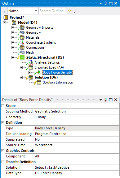
For a structural analysis you can import Imported Body Force Density (illustrated below) and Imported Surface Force Density load types.
Add the Imported Load
Follow these steps to add an imported load and associate it with parts of the geometry.
Double-click the Model cell in your analysis system to open the Mechanical application.
Click the Imported Load group object. In the Details view, set the following field as needed:
If you want to suppress all of the loads under this Imported Load group, set the Suppressed field to .
For the Body Force Density and the Surface Force Density loading types, you can choose to import the or the , if the source provides the data, using the Data Type property. By default, the application imports the values. The application combines AC and DC values to calculate the value. Because the AC force is a complex vector, the peak vector among all phases of the AC force is taken and added to the DC force to obtain the .
There are several ways to select an imported load and associate it with a part of your model.
Select an Imported Load group object in the tree, select a part of the model, then right-click and from the menu, select the desired load type. The load will be applied to the object you selected on the model.
Click an Imported Load group object in the tree, then select the Imported Loads drop-down menu on the Context tab and select the desired load type from the allowed imported load types. In the Details view, click the Geometry field. Select the objects in the model to which you want to apply the load and click the button in the Geometry field.
Right-click the Imported Loads group object and select and the desired load type from the allowed imported load types. In the Details view, click the Geometry field. Select the objects in the model to which you want to apply the load and click the button in the Geometry field.
Note: Heat generation loads scoped to a surface body use the constant thickness value specified in the details view of the surface body object when data is imported. Surface body thickness defined using the thickness object is not accounted for when data is imported.
Set the Imported Load Options
Click the imported load object that you've added to the tree.
Select the desired Ansoft solution you would like to import the load from. Some of the properties in the Details view and Data View tab are filtered based on this selection.
Change any of the fields in the Details View as needed:
Scoping Method: Select the method of choosing objects to which the load is applied: Geometry Selection or Named Selection.
Geometry or Named Selection: Use these fields to choose the objects to which the load is applied, as appropriate from your Scoping Method choice.
Suppressed: Select Yes to suppress this load.
Ansoft Surface(s): Select the Ansoft Surface(s) for a Heat Flux or Surface Force Density load.
or
Ansoft Volume(s): Select the Ansoft Volume(s) for a Heat Generation or Body Force Density load.
Set the Imported Load Analysis Options
You can specify when the imported data should be applied and also modify the imported data, either by adding an offset or by using a scale factor.
To see the analysis setting for a load, click the object that you've added to the tree. The analysis options appear in the Data View tab of the window below the model. Make any changes to the load's analysis options as indicated below.
Change any of the columns in the Data View tab as needed:
Source Frequency - Select from the drop-down list one of the frequencies supplied from the transfer file. The load values associated with this frequency will be imported.
Source Time - Select from the drop-down list one of the Source Times supplied from the transfer file. The load values associated with this time will be imported.
For thermal loads from Maxwell transient solutions, you must select from the drop-down list the desired Source Start Time and Source Stop Time to define the interval for integrating the power loss density distribution.
Analysis Time - Choose the analysis time at which the load will be applied. This must coincide with the end time of a step defined in the Analysis Settings object in the tree.
Scale - The amount by which the imported load values are scaled before applying them.
Offset - An offset that is added to the imported load values before applying them.
You must re-solve after making any changes to the analysis options of a load.
You can define multiple rows in the Data View tab to import additional data from the selected Ansoft solution and apply the rows at different analysis times. If multiple rows are defined in the Data View tab, you can display imported values at different time steps by changing the Active Row option in the Details pane.
Right-click the Imported Load object and click Import Load to import the load. When the load has been imported successfully, a contour plot of the temperatures will be displayed in the Geometry window and a summary of the transfer is displayed as a comment in the particular load branch.