


For this probe, result “positions” are created for time points along selected coordinate system axis or axes. These result values are plotted in the Graph window. This probe must be scoped to a rigid body. It is supported for Static Structural, Transient Structural, Rigid Dynamics, and Explicit Dynamics analyses.
Using the result values in Tabular Data, you can animate the scoped body in motion. In addition, if you set the Result Selection property to , the Position probe provide a unique graphical display feature. It displays a “trace” or red line that follows the movement of the scoped body. The trace is based on the result values of the scoped body for all three axes over time (as contained in Tabular Data). The example below shows a rotation. Linear movements are also supported. The small red ball shows the current position along the curve.
Rigid Dynamics Solver
With the Rigid Dynamics Solver, the position probes can also be used to report the location of the resulting contact force. In order to get the contact force location, the Location Method field must be set to Contact Region. Then the Contact Region drop-down allows you to select the contact region for which the position will be reported.
Note: Contact regions between the same pair of parts are merged into a single contact region. Consequently, the probes will report the same values for the entire contact region.
If the contact is open, the position probe will report zero for all components, leading to abrupt jumps to the global origin in the trajectory plot. In some situations, the position probe seems to report erratic location information. Typically, in a cylinder/plane frictionless contact, the contact forces/torque can be equally reported anywhere along the contact line as in (a) below. The position in the plane perpendicular to the contact line is perfectly consistent in that case as in (b) below.
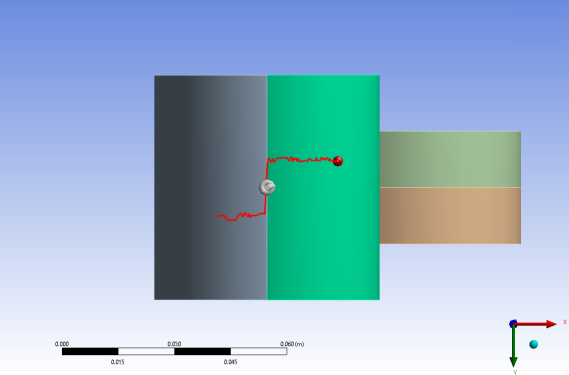 (a) contact probe viewed in X-Y |
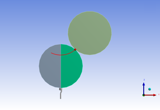 (b) contact probe viewed in X-Z |